Forecast Method Parameters
Each Forecast Method has unique parameters. The following are the definitions for each parameter included in the system:
Alpha
Affects the estimate of the intercept.
Arima
- ArimaD: Number of times to difference the series.
- ArimaP: Autoregressive order.
- ArimaQ: Moving average order.
Beta
Affects the slope.
Cycle
Each seasonal method needs to know how many forecasting periods belong to a year. Usually this is 12, sometimes 4 or 52.
The forecasting engine looks for the number in the cycle parameter to gauge seasonality, so it is very important to update the cycle parameter accordingly.
For example, in a monthly bucket data set if a data set repeats every 8 months then the Demand Planner needs to set the cycle to 8. If a data set repeats every 7 days in daily buckets then the cycle parameter needs to be set to 7, etc. These buckets are defined in the Edit window of the forecast view.
Damping Factor
Damping factor attempts to damp linear data. This parameter affects methods which forecast a trend. The trend is normally a fixed amount T that is added to the forecast each period. For a series without longstanding history, continuing the trend into the future can often be overly optimistic or pessimistic. When the damping factor is set to something less than 1, the steps are successively reduced in size by multiplying by successive powers of the damping factor. For example, if the damping is 0.9, then the successive steps are T, 0.9T, 0.81T, 0.73T, 0.66T, etc. The resulting forecast is a curve with slope decreasing in size.
🚧 Warning
Do not set Damping Factor to 1.
Event Factors
Even factors are calendar periods of events that may influence the trend or direction of a time series occurs. It is used to minimize the impact of events on forecasting.
Units and Direction
These parameters affect the Unitizing process, which is an extra step that happens after all forecasting is completed. To turn off unitizing, keep the Units parameter at its default value of 0.0. To run unitizing, enter a positive value for the Units parameter. The original forecast will then be modified so that each value is an integer multiple of the Units parameter.
For each forecast value, there will usually be a remainder — an extra fraction of a Unit — which could be rounded up or down. When the Direction parameter is kept at 0.50, an extra amount totaling 0.50 Units or more will be rounded up to an additional Unit. This can be relaxed by setting the Direction parameter, so that, for example, if Direction = 0.25 then anything exceeding 0.25 Units will be rounded up to an entire additional Unit.
Gamma
Affects the correction terms.
Innovation
Early adopters. The probability or rate at which an innovator buys the product in a period.
Imitation
The probability that an imitator adopts the new product. Also called Contagious Effect.
Lag
This affects exponential smoothing, both single and double. It determines the length of the window of recent history that is used in forecasting. For example if theta equals 0.1, then the weights are successive powers of (1 – 0.1) = 0.9, namely 1, 0.9, 0.81, 0.73, 0.66. 0.6, 0.53, etc. When Lag = 5, for example, only the first 5 of these are used.
Lag can be large (for example, 10 or 12) when a series has a long stable history. Smaller values work better for a short volatile series.
MarketSize
Number of adopters or potential Market over the life of the product.
MaxPctPos
This is the fraction of historic values that can be positive and still pass the test; defaulted to 0.6. Anything more than 0.6 and it will revert to exponential smoothing. Leading zeroes are not counted for this.
MultiRegWeight
This parameter affects methods which forecast via regression. Ordinary regression (with this parameter set to 1) puts equal weight on fitting all past values of the series. When this is set to something less than (but close to) 1, the weights decrease back into the past.
For example, if MultiRegWeight = 0.95, Then the weights of successive values moving back into the past are 1.0, 0.95, 0.9, 0.86, 0.81, 0.77, 0.74, etc. For a volatile series, this could improve the fit, while it will worsen the fit in the case of a series with a long stable history, Number of Weights: Set number to add more weights than the default 5.
🚧 Warning
Do not set regression weights to 1.
NumberOfWeights
The number of periods for which weights would be applied, applies to the outlier method.
Offset
This affects several smoothing methods (Three Span Median, Average, Single Exponential, Weights). For forecasting, this parameter should always remain at its default value of 0.
In special cases, these methods can also be used to smooth a series rather than forecast it. This can be done by giving Offset a negative value, which has the effect of moving the output that many periods backwards into the past.
For example, Three Span Median normally puts the median of the n, n+1, and n+2 values as a forecast for the n+3 position. However, when Offset = -2, this median is put in the n+1 position, where it replaces the n+1 value with the median of itself and its neighbors. In more general cases, usually Offset = – (Ceiling(lag/2)) or Offset = – (Ceiling(NumberOfWeights/2)).
The double smoothing methods can’t be used in this way. Offset can be kept at 0, as it has no effect.
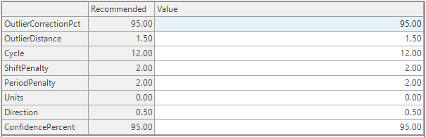
Outlier
The Outlier_Method in Stat Forecast is used to identify unusual peaks and valleys (outliers) in the data. Further, it can be used to smooth/correct the history as well. This is useful where the data has a lot of spikes caused by events/factors that do not have a good possibility of re-occurring. A best practice might be to simply identify the outliers, and selectively weed out the ones that fit the given parameters.
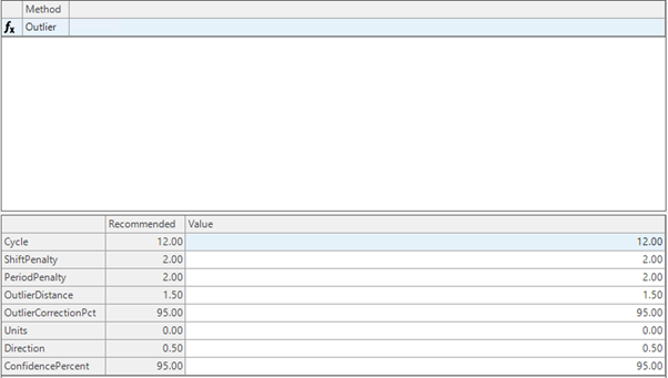
Parameters
- Cycle: Number of Periods – 12 -for monthly or 52 for weekly
- ShiftPenalty: This parameter is capable of detecting a “level shift” where there is a one-time increase of decrease in the overall level of the series. It can also detect if there is a single month where the series has a seasonal adjustment that departs from the sine and cosine curves that the model is trying to fit.
- PeriodPenalty: If the “penalty” for one of these effects is high — at the default value of 2.0 — then it will not affect the result. If the penalty is reduced to 1.5, the given effect can come into play. In order for the penalties to be lowered, there should be at least several years of history in order to estimate the underlying trend and seasonality
- OutlierCorrectionPct: correction percentage when outlier is detected
- OutlierDistance: A value used to determine outlier limits
The outlier method starts by fitting a robust seasonal to the data. It then calculates the residual errors for the observations and finds the inter-quartile range of the errors to get an estimate of the standard deviation. The inter-quartile range is not as affected by extreme errors as the usual sample standard deviation. Each data point is evaluated on being within the specified distance (the default of 1.5 is equivalent to 2 standard deviations). Values falling outside that range are corrected to the correction percent, e.g. the default of 95 will move the observation 95% of the way to the outside range of errors.
The outlier analysis is based on the below steps:
- Run Robust seasonal forecast method to get a forecast
- Obtain residuals using the forecast obtained by Robust-Seasonal method i.e Actual History- Forecast
- Obtain the Q3 and Q1 quartile values from the residuals – the excel has the formula for Q3 and Q1
- calculate IQR=Q3-Q1
- Apply Q3+1.5_IQR and Q1-1.5_IQR to get the upper and lower cutoff points(1.5 IQR is equivalent to 2sigma limits i.e 95% of the data)
- Any residual from step 2 that falls outside of upper and lower cutoff points from step5 will be marked as outlier
- This link has the same steps :https://documentation.arkieva.com/docs/practical-application
📘 Note
We suggest the Outlier be run at the level at which forecast accuracy is computed.
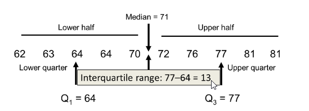
Quartiles
- Quartiles divide the entire set into four equal parts. So, there are three quartiles, first, second and third represented by Q1, Q2 and Q3, respectively. Q2 is nothing but the median, since it indicates the position of the item in the list and thus, is a positional average. To find quartiles of a group of data, we have to arrange the data in ascending order.
- First quartile (Q1), also known as lower quartile, splits the lower 25% of data. It is the middle value of lower half.
- Second quartile (Q2) which is more commonly known as median splits the data in half (50%). Median divides the data into a lower half and an upper half.
- Third quartile (Q3), also known as upper quartile, splits lowest 75% (or highest 25%) of data. It is the middle value of the upper half.
- The first quartile is also known as 25th percentile, the second quartile as 50th percentile, and the third quartile as 75th percentile.
- The Interquartile range (IQR) is from Q1 to Q3. It is the difference between lower quartile and upper quartile.
- IQR = Q3 – Q1
Residuals
The “residuals” in a time series model are what is left over after fitting a model. For time series models in demand planning, the residuals are equal to the difference between the Actual Sales History and the corresponding forecasted value.
Example
| Month | Sales Volume | Forecast | Residual |
|---|---|---|---|
| Jan-2022 | 400 | 375 | 25 |
| Feb-2022 | 500 | 520 | -20 |
| Mar-2022 | 380 | 400 | -20 |
| Apr-2022 | 420 | 410 | 10 |
Outlier Calculation Examples
Example 1
No outliers here for example 1 since all residuals fall within the lower and upper limits.
| Q3 | Q1 | IQR |
|---|---|---|
| 7954 | -488 | 8402 |
| Data | Sales History | Generated Forecast - RobustSeasonal | Residual | Upper Limit | Lower Limit |
|---|---|---|---|---|---|
| 9/1/2020 | 28000 | 9470 | 18530 | 20557 | -13051 |
| 10/1/2020 | 0 | 0 | 0 | 20557 | -13051 |
| 11/1/2020 | 0 | 0 | 0 | 20557 | -13051 |
| 12/1/2020 | 0 | 4819 | -4819 | 20557 | -13051 |
| 1/1/2021 | 18000 | 10238 | 7762 | 20557 | -13051 |
| 2/1/2021 | 0 | 11637 | -11637 | 20557 | -13051 |
| 3/1/2021 | 28000 | 8254 | 19746 | 20557 | -13051 |
| 4/1/2021 | 0 | 3637 | -3637 | 20557 | -13051 |
| 5/1/2021 | 18000 | 3637 | 14363 | 20557 | -13051 |
| 6/1/2021 | 0 | 3637 | -3637 | 20557 | -13051 |
| 7/1/2021 | 18000 | 11793 | 6208 | 20557 | -13051 |
| 8/1/2021 | 18000 | 100000 | 0 | 20557 | -13051 |
| 9/1/2021 | 18000 | 9470 | 8530 | 20557 | -13051 |
| 10/1/2021 | 18000 | 0 | 18000 | 20557 | -13051 |
| 11/1/2021 | 0 | 0 | 0 | 20557 | -13051 |
| 12/1/2021 | 10000 | 4819 | 5182 | 20557 | -13051 |
| 1/1/2022 | 18000 | 10238 | 7762 | 20557 | -13051 |
| 2/1/2022 | 8000 | 8000 | 0 | 20557 | -13051 |
| 3/1/2022 | 0 | 4617 | -4617 | 20557 | -13051 |
| 4/1/2022 | 0 | 0 | 0 | 20557 | -13051 |
| 5/1/2022 | 10000 | 0 | 10000 | 20557 | -13051 |
| 6/1/2022 | 0 | 0 | 0 | 20557 | -13051 |
| 7/1/2022 | 0 | 1793 | -1793 | 20557 | -13051 |
| 8/1/2022 | 0 | 0 | 0 | 20557 | -13051 |
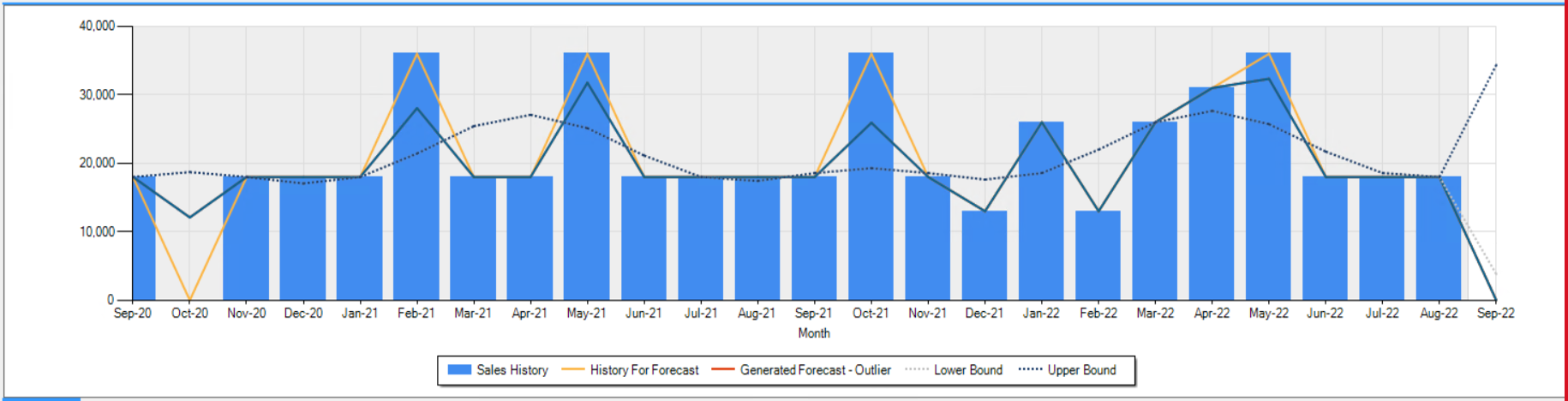
Bold marked values in the Residual column are the outliers here since these residuals fall outside the upper and lower limits.
| Q3 | Q1 | IQR |
|---|---|---|
| 1543 | -3277 | 4821 |
| Data | Sales History | Generated Forecast - RobustSeasonal | Residual | Upper Limit | Lower Limit |
|---|---|---|---|---|---|
| 9/1/2020 | 18000 | 18000 | 0 | 8775 | -10509 |
| 10/1/2020 | 0 | 18720 | -18720 | 8775 | -10509 |
| 11/1/2020 | 18000 | 18000 | 0 | 8775 | -10509 |
| 12/1/2020 | 18000 | 17055 | 944.8 | 8775 | -10509 |
| 1/1/2021 | 18000 | 18000 | 0 | 8775 | -10509 |
| 2/1/2021 | 36000 | 21430 | 14570 | 8775 | -10509 |
| 3/1/2021 | 18000 | 25428 | -7428 | 8775 | -10509 |
| 4/1/2021 | 18000 | 27088 | -9088 | 8775 | -10509 |
| 5/1/2021 | 36000 | 25141 | 10859 | 8775 | -10509 |
| 6/1/2021 | 18000 | 21134 | -3134 | 8775 | -10509 |
| 7/1/2021 | 18000 | 18000 | 0 | 8775 | -10509 |
| 8/1/2021 | 18000 | 17428 | 572 | 8775 | -10509 |
| 9/1/2021 | 18000 | 18572 | -572 | 8775 | -10509 |
| 10/1/2021 | 36000 | 19293 | 16707 | 8775 | -10509 |
| 11/1/2021 | 18000 | 18572 | -572 | 8775 | -10509 |
| 12/1/2021 | 13000 | 17628 | -4628 | 8775 | -10509 |
| 1/1/2022 | 26000 | 18572 | 7428 | 8775 | -10509 |
| 2/1/2022 | 31000 | 22002 | -9002 | 8775 | -10509 |
| 3/1/2022 | 26000 | 26000 | 0 | 8775 | -10509 |
| 4/1/2022 | 31000 | 27660 | 3340 | 8775 | -10509 |
| 5/1/2022 | 36000 | 25714 | 10286 | 8775 | -10509 |
| 6/1/2022 | 18000 | 21707 | -3707 | 8775 | -10509 |
| 7/1/2022 | 18000 | 18572 | -572 | 8775 | -10509 |
| 8/1/2022 | 18000 | 18000 | 0 | 8775 | -10509 |
OutlierCorrectionPct
Correction when outlier is detected, applies to the outlier method.
OutlierDistance
A value used to determine outlier limits, applies to the outlier method.
PeriodsToAverage
Number periods to average, applies to the average method.
PeriodPenalty
Robust Seasonal; look for periodicity in history.
R method parameters
The following are exclusive forecast parametes to R methods.
R is an open source Statistical software package. R integration objective is to extend Arkieva’s forecasting functions to include forecasting Methods from R. The R integration currently is not optimized for speed. The added functions include Arima and intermittent functions. The new forecasting functions would be included with forecasting options available in Arkieva. The new additions are RArima, RAutoArima and Rintermittent.
Install R
R must installed along with the Arkieva application. From the Arkieva installation window, select “R for windows” link to install R. Once R is installed, from you start menu invoke R and type the following commands:
- Install.packages("forecast")
- Install.packages("TSA")
- Install.packages("tsintermittent")
Event Factors
This allows the effects of the event to be included in the model. The events sometimes may change the direction of the historical trend. The impact of an event may be short term or linger for some time. The set up for the event factors is like the setup for the Regression Method in Arkieva. Event factors may be a onetime activity or multiple activities.
If the effect of the event is temporary and decay over time, then the period of the event is assigned a 1 and all other periods are assigned 0.\ If the effect of the event is permanent over time, then the period of the event and future periods are assigned a value of 1 and all other periods are assigned a value 0.\ Where we have multiple events within the historical time horizon, then a column must be created for each event.
Regression factors
These may be variables that has some relationship with the historical data. This is included in the model when trends alone in the historical data are not sufficient for a good fit for the model. To use regression factors, we need not only the historical data but also future regression factors to accurately forecast future activities. We can have at least one regression factor, R would decide with of the factors are significant to be included in the model. The set up for the event factors is like the regression factors setup with the Regression Method in Arkieva.
R Arima
R-Arima is also a Regression based model that is the preferred method for sales which are not trending; i.e. trending high or low but shows stable range for average and has some peaks. This is in case we have less information about the sales but we see a good spread overall through the time series.
Hence it is useful for any certain event in the future like in the past; i.e. Christmas, promotion, special days, etc., have normal sales also included.
Requirements
- Dummy Variable (optional): You would need to specify or pin point those events in the past by using a dummy variable like 1,0,1,0, and periods in the future where you would expect them to repeat.
- Event Factor (optional): if you could identify the events in the past and are not expected to occur again, i.e. you want them to be excluded before forecast.
- Create a quantity for it and publish the dummy variables using a function that can identify peaks. (i.e. insert 1 if the sales is 10 x of base sales else 0)
- Provide source table and column and Date like usual quantities.
- Assign that quantity as factor under usage in SETUP Manager.
- Select Forecast and Regression and click Apply.
Factors\ They range from (0,1,2) except cycle.
- Cycle = number of time buckets in a year cycle; i.e. 52 for weeks, 12 for monthly data set
- Arima P = Auto regressive parameter.
- Arima D = Difference; 1 means to reduce the data by 1 lag to stabilize the data.
- Arima Q = Moving average; fixing error 1 lag at a time.
- Arima SP = Seasonal Parameter
- Arima SD = seasonal difference; to reduce the data by one cycle i.e. 52 weeks or 12 months. Considers the difference of 2 data points in each season.
- Arima SQ= seasonal moving average; it tries to adjust the future predictions based on what it has done in the past year during each season.
Select Type
Default value is 1 (Crosston Method). Changing the value to 2 creates a generalized method that automatically selects the optimal method and parameters.
MaxAI
The Max aggregation level, the default is the number of historical periods.
MinAl
The Minimum aggregation level, the default value is 1.
MaxPctpos
For checking if the data is sporadic. Takes values between 0 and 1; the default is 0.6.
Comb
Default value is the “mean”: 1 for Mean, 2 for Median.
Regression Factor
- Regression Factors: these are the external factors used in Multiple Regression Method.
- Regression Factor Values: The actual values associated with each factor.
- Regression Factor Offsets: These are positional shifts within a factor.
ShiftPenalty
SporadicOption
Sporadic Option determines how to handle a situation where it has been too long since the last observation, meaning the estimate of the next observation has already passed.
- Option 0 is to keep using the same method – exponential smoothing
- Option 1 is to ignore the ending zeros and forecast the same
- Option 2 is to copy the historic values into the future
- Option 3 is to forecast as if the next observation will come in the first future bucket and then modify the future interval estimates accordingly
Syntetos-Boylen
Un-biasing for Croston (0 or 1).
Theta
Parameter that appears in multiple Methods.
- Croston: smoothing parameter.
- Double exponential: data smoothing parameter.
- Single exponential : Smoothing parameter.
- Sporadic: Smoothing parameter.
🚧 Warning
Do not set the Theta to 0.
Related Articles
Statistical Forecast
Introduction What is Statistical Forecasting? Statistical Forecasting is one of the components of the overall Arkieva Demand Planning process. The purpose of the Demand Planning process is to create an Unconstrained Consensus Demand Plan from the ...Forecast Performance
The following is a list of Performance Metrics. Bias Total bias shows how many units your forecast is deviating from the actual sales values in absolute terms and whether the forecast is biased towards overestimating or underestimating the actual. ...Forecast Methods
Introduction To create a custom method to be used in the Statistical Forecast component, click the New button located in the Forecasting Methods ribbon. The new method with the name 'New Method' will appear under the Custom Methods category. Under ...Forecast Formulas
When selecting a formula, the associated methods will be highlighted under the Method section. Smoothing Formulas The Smoothing Formulas are 3_Span_Median_S, Average_S, and Weights_S. For forecasting highly variable series, a method can be defined ...Forecast Performance Management
“What gets measured, gets managed.” There are a many alternatives on how to measure forecast accuracy. It does not matter too much how you define the KPI as long as: it is consistent, and it is understood by all stakeholders. Therefore, choose a set ...