Forecast Performance
The following is a list of Performance Metrics.
Bias
Total bias shows how many units your forecast is deviating from the actual sales values in absolute terms and whether the forecast is biased towards overestimating or underestimating the actual. This could be interesting for showing the evolution of the deviation over time but comparing different results across products, forecast techniques… is difficult to accomplish by this metric.
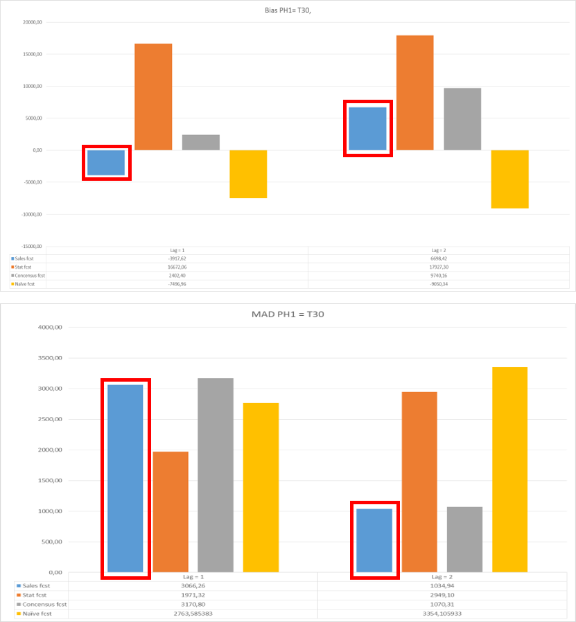
Calculating the total sum of the deviations or calculating the mean can give you an overall image of the evolution. However, this sum or mean cannot be used as a representative metric to verify how well the forecast is performing. E.g. it might be possible that a forecast technique that has a small absolute error, gives a higher total bias value than a technique with large opposite deviations. In the latter case, these large opposite deviations cancel each other out. In the figure below, the metric bias is compared to the MAD.
The sum of the bias suggests that the forecast of lag one is better than the forecast of lag two, because it has a lower absolute value. However when looking at the MAD, we can see that it is the other way around: the forecast used on the second lag is better since its absolute deviation is closer to zero.
🚧 Limitation
Not able to perform cross item comparisons.
NFM (Normalized Forecast Metric)
This metric will stay between -1 and 1, with 0 indicating the absence of bias. Consistent negative values indicate a tendency to under-forecast, whereas consistent positive values indicate a tendency to over-forecast. Over a 12 period window, if the added values are more than 2, we consider the forecast to be biased towards over-forecast. Likewise, if the added values are less than -2, we consider the forecast to be biased towards under-forecast.
MSE (Mean Squared Error)
Same usage as the MAD. The elimination of negative values is obtained by using the square function. The error is expressed in squared units.
🚧 Limitations
Since it is a scale dependent metric, this is not appropriate to compare different time series with each other. However this metric can be used to compare different forecasting techniques on the same dataset. Sensitive to outliers (because of the square term).
RMSE (Root Mean Squared Error)
See MSE. Basically the same interpretation possible.
🚧 Limitations
Sensitive to outliers. Scale dependent metric; only able to compare different forecast techniques on the same dataset.
MPE (Mean Percentage Error)
PE is in fact more or less the same as APE, with the sole difference that this metric will work with the exact values and not with the absolute values. As is the case with bias, this can be used to look if the forecast is biased toward underestimating or overestimating the actual values.
🚧 Limitations
Cannot cope with zero actuals. Therefore, this metric is not ideal for analyzing intermittent demand patterns.
MASE (Mean Absolute Scaled Error)
MASE will compare the MAD of the used forecast method with the MAD of the naive forecast. Notice that the MAD of the naive forecast start at t=2 (in case of lag 1), since the first naive forecasted value cannot be assigned.
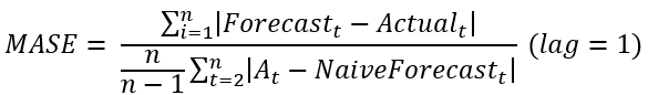
When the MASE value is less than 1, the forecast is better than the naive forecast. Otherwise the naive forecast is better than the used forecast technique.
This scale-free error metric can be used to compare forecast methods on a single series but also to compare forecast accuracy between series. This metric is well suited to intermittent-demand series because it never gives infinite or undefined values except in the irrelevant case where all historical data are equal. This metric can cope with trend patterns and seasonality.
🚧 Limitations
MASE is more difficult to understand by business users. In academic context it is often used as the reference metric since it is perceived as the best measure of forecast accuracy.
U-statistic (Theil’s U statistic)
The U-statistic is a relative metric, which means it is scale independent and can thus be used for comparing different datasets with each other. It compares the forecast technique with the naive forecast. If the U value is equal to 1, the forecast has the same performance as the naive forecast. When it is less than 1, the used forecast technique is better than the naive forecast.
🚧 Limitations
Outliers are taken into account.
Tracking signal
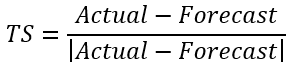
Tracking signal is used to verify whether a forecast technique is unbiased. There are control limits (e.g. ±2, ±4 are most used) to monitor the bias of the forecast. In this metric, the sum of errors is measured as a percentage of the MAD. Although the MAD is large, when the sum of the errors is rather small, then you can conclude that the forecast is unbiased (over forecasting compensates under forecasting). If the sum of the errors increases, that means that there is a systematically over/under forecasting, the TS becomes larger. In the latter case, the used forecasting technique should be reviewed.
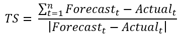
Figure 1: Example calculation of Tracking Signal
📘 Alternative formula
The “Tracking Signal” quantifies “Bias” in a forecast. No product can be planned from a badly biased forecast. Tracking Signal is the gateway test for evaluating forecast accuracy. The tracking signal in each period is calculated as follows:
📘 Note
Once this is calculated, for each period, the numbers are added to calculate the overall tracking signal. A forecast history totally void of bias will return a value of zero, with 12 observations, the worst possible result would return either +12 (under-forecast) or -12 (over-forecast). Generally speaking such a forecast history returning a value greater than 4.5 or less than negative 4.5 would be considered out of control.
Rules Method
This is a dynamically generated rule-based forecast. The rules are created based on the unique trends in the data. It looks for similar trend occurrences in the data and summarizes the data that has similar trends to represent the trends. For example, if a customer buys a product every Tuesday and Thursday, 10 units every Tuesday and 20 units every Thursday, then the rule apply 10 units to every Tuesday and 20 unit every Thursday. If a company does not operate on weekends, then the rule would recognize that and ensure the rule is honored. If the company used to work on weekends but no longer does, then in some instances the rule would recognize this change.
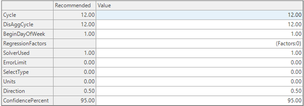
The rule logic is now available in Arkieva as a formula call the “RuleSForecast”. It has the following parameters:
- Cycle; the number of periods in a year
- DisAggCycle; Higher level period aggregation, for example Weekly or Monthly
- BeginDayOfWeek: Beginning Day of the Week, this only applies when DisAggCycle is Weekly. 0 is Sunday and 6 is Saturday.
- Regression Factor: this provides the ability to include Regression Factors as an additional input.
- SolverUsed; different logic available.
| 0. | Rule + Disaggregation: in addition to the rules forecast, data is also aggregated to a higher level, forecasted, and disaggregated back to the original level of the data |
| 1. | Rule + Factors: would include regression factors if available |
| 2. | Rule + Disaggregation: in addition to the rules forecast, data is also aggregated to a higher level, forecasted, and disaggregated back to the original level of the data |
| 3. | RuleRatio: estimates lower-level proportions from higher level aggregation |
| 4. | Next Event: |
- Error Limit: The rules formula sometimes overfit the model, this is a situation where we have a good fit but not so good forecast in the future. If the value is too large the model is close to the average of the data, if it is too small the model does not change.
- SolveType: aggregation of the response variable when rule conditions have been met.
| 0. | Avg: Average of the response |
| 1. | Median: Median of response |
| 2. | - TrimAvg: Trim Average of the response |
| 3. | Percentile: 90th percentile of response |
Has ability to handle any data that has a structured trend. Below are some sample forecast results:

Plain forecast
Smart Forecast:
Rules Forecast:\ Parameters: Cycle =12, solver used=1, error limit=0
Using Regression Factors
Multiple Regression: using Factors
Rules Forecast Using Only Regression factors:\ Parameters: Cycle =12, solver used=4, error limit=0
Rules Forecast using Factors Plus internal data trend:\ Parameters: Cycle =12, solver used=2, error limit=0
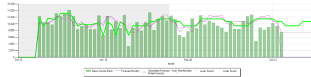
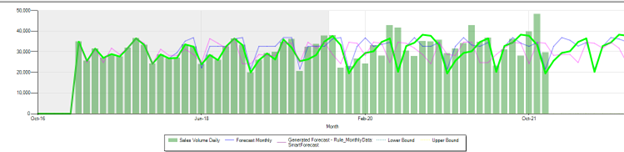
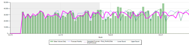
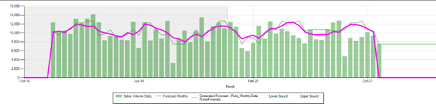
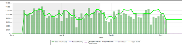
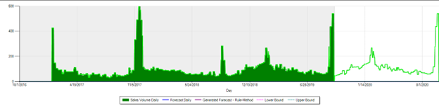
Daily Forecast:\ Daily Forecast has a lot of variability and the seasonal period do not line up from season to season and there are very difficult with traditional methods. Here are examples of daily forecast using Rules Forecast.\ Parameters: Cycle =365, solver used=1, error limit=0
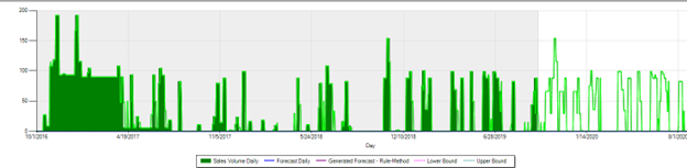
Parameters: Cycle =365, solver used=1, error limit=0
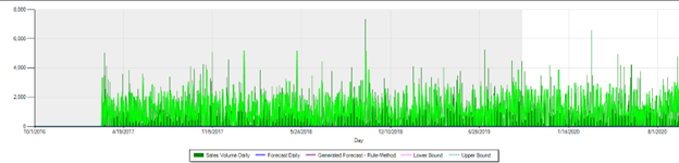
Parameters: Cycle =365, solver used=1, error limit=0
Related Articles
Forecast Performance Management
“What gets measured, gets managed.” There are a many alternatives on how to measure forecast accuracy. It does not matter too much how you define the KPI as long as: it is consistent, and it is understood by all stakeholders. Therefore, choose a set ...Forecast Methods
Introduction To create a custom method to be used in the Statistical Forecast component, click the New button located in the Forecasting Methods ribbon. The new method with the name 'New Method' will appear under the Custom Methods category. Under ...Statistical Forecast
Introduction What is Statistical Forecasting? Statistical Forecasting is one of the components of the overall Arkieva Demand Planning process. The purpose of the Demand Planning process is to create an Unconstrained Consensus Demand Plan from the ...Forecast Formulas
When selecting a formula, the associated methods will be highlighted under the Method section. Smoothing Formulas The Smoothing Formulas are 3_Span_Median_S, Average_S, and Weights_S. For forecasting highly variable series, a method can be defined ...Forecast Netting
The netting process evaluates which part of the forecast has not been ordered or shipped yet. The outcome of the process is a remaining forecast in daily buckets. Normally this aggregates back up to the time level (week, month) that the planning is ...