Forecast Methods

Introduction

To create a custom method to be used in the Statistical Forecast component, click the New button located in the Forecasting Methods ribbon.

The new method with the name 'New Method' will appear under the Custom Methods category.

Under the Method Properties section, type a name for the new Custom Method.

The name typed will be reflected automatically under the Custom Methods category.

Optionally, type an explanation for the custom method in the Description field.

Under the Method Definition section, add the formula to be included in the custom method by either double-clicking them from the formula list or clicking once and clicking the Arrow key. Reorder the formulas in the Included Items box with the Up and Down Arrows.

You can also optionally double-click under the Value column to edit formula values.

Next, select an Error Measure and Select the number of periods from the Comparison Window section. The Comparison Window is the number of most recent time periods that the forecasting methods will simulate as future to determine the accuracy of the forecast. Values from 3 to 6 usually work well, with the larger values being appropriate when there is more (>24 months) stable history to base forecasts on.

Checking the Flexible checkbox will change the Comparison Window to a Dynamic Window.The Methodology dropdown is where you will select formulas to include in the custom method.

When finished, save the custom method by clicking the Save button located in the toolbar. The asterisk next to a custom method means that any changes made have not be saved.

The custom method will now be available in the Statistical Forecast.

Each method is a list of one or more formulas together with a specific choice of parameters for each formula.

Method Aggregation

Smart Forecast method

The smart method is capable of handling almost all types of time series data. All that is required is time series data and the number of periods in a year (cycle). The method takes complete control as to which methods are used and the values of the parameters used. The smart method can be seen as a Blackbox; the only information provided is the forecast. It does not provide information on which methods were used or which method was selected.

Smart forecasting goes through the following steps:

Classification or identification: identifies the type of time series; e.g. seasonal, intermittent, etc.
Selects a list of methods that matches the identified classification.
Selects the method that gives the best error. There are options that allow for some form of stitching of the outputs of the different methods to generate a better outcome.

Class of time series data: any type of time series data. Can be used in almost any situation, however it is best utilized when knowledge of time series forecasting is limited.
Setup: The only parameter that requires review is the cycle.
Competitiveness: Smart method is very competitive against any method but possible to generate a better result manually (time consuming for similar results).

Parameters\ Cycle (required): Number of periods in a year, weekly=52, monthly=12, quarterly=4\ Select Type (default is Normal):

Normal: Determines classification type then gets the set of associated methods. Based on classification it selects the best method from the selected list. List of required methods are generated by the system.
Average: Uses the list of methods generated in the normal type and implements the average methodology.
Minimal: Uses the list of methods generated in the normal type and implements the minimal methodology.
Regression: Uses the list of methods generated in the normal type and implements the Regression methodology.
Ridge: Uses the list of methods generated in the normal type and implements the ridge regression methodology.
Lasso: Uses the list of methods generated in the normal type and implements the Lasso methodology.
Quantile: Uses the list of methods generated in the normal type and implements the Quantile Regression methodology.
All: Implements all the above methods from 0 to 6 and then and picks = best solution.\ Data label: Determines the time series classification. Default = unknown, selects from the list if the classification is known.\ Remove Outliers: Ability to detect and remove outliers. Default is False.

Probabilistic Forecast method

Probabilistic forecast method can be used for any time series.

Parameters

Regression Factors

The external factors used as in Multiple Regression Method.

Regression Factor Values

The actual values associated with each factor.

Regression Factor Offsets

Positional shifts within a factor.

Cycle

Number of periods in a year: weekly=52, monthly=12, and quarterly=4.

Select Type

Quantile Regression approximation.
Normal distribution approximation.

Number of Percentile

The number of percentiles generated for interpolation; not needed if quantile option is selected.

First Probability

Probability for the first band.

Second Probability

Probability for the second band.

Gradient Boost method

Parameters

Cycle

Number of periods in a year: weekly=52, monthly=12, and quarterly=4.

Iterations

Maximum number of iterations; actual iterations may be lower than this value. Higher iterations results in more run time.

Regression Factors

The external factors used as in Multiple Regression Method. If factors are not provided one is generated through Smart logic.

Regression Factor Values

The actual values associated with each factor.

Regression Factor Offsets

These are positional shifts within a factor (currently not linked).

Trend methods

Time Series in history helps to understand if series are going up or going down. Delta (Trend) is calculated by taking the difference of each period with its previous period.

I.e. In below example delta values are calculated as:

For Period = -13, Delta = (102 - 111) = -9
For Period = -12, Delta = ( 105 - 102) = 3
For Period = -11, Delta = ( 100 - 105) = -5 and so on

If delta values are positive for the entire history, then it means that the trend is increasing:\ I.e. Positive Trend

Like-wise if the delta values are negative for entire history, then it means that trend is decreasing:\ I.e. Negative Trend

The set of formulas used for trend methods are dependent on 2 things:\ I.e. History and Delta values.

🚧 Warning

These methods need to be controlled by a damping factor – The reason being the forecast growing limitless into millions or infinity needs be pulled down and the forecast that is decreasing needs to be pulled up.

Double Exponential Smoothing\ Double Exponential Smoothing is a trend method that tries to fit a curve. It fits a trend to recent history from the most recent 2k-1 values, where k is equal to the value of the Nmb_of_Wghts parameter. Set k to 6 or more in order that a reasonably long window is used to estimate the trend. Parameter Theta determines the relative weight of more recent versus less recent history, as with the Single_Exp formula.

Set Theta equal to a small value near 0, in the .05 to .20 range. Larger values of Theta place more weight on recent history. The Damping parameter should be between 0.9 and 1.

This method is similar to single exponential method that uses parameter to apply the weights to past periods.

Calculation: If theta parameter is set to 0.15 then immediately preceding period to current period will get full weight I.e. 100%.

Period which is 2 periods prior will get 85%,
Period which is 3 periods prior will get 72%.

According to which weights applied are 39%, 33% and 28% respectively.

Forecast generated for Current Period is 151.27 which is the weighted average of 148, 152 and 153.

I.e. 148_0.28 = 41.44, 152_0.33 = 50.16, 153*0.39= 59.67, then calculate:\ SUM = 41.44 + 50.16 + 59.67 = 151.27.

Like-wise the mean delta value is 3.11 which is the weighted average of 5, 4 and 1.\ I.e. 5_0.28 = 1.4, 4_0.33 = 1.32, 1*0.39= 0.39, then calculate:\ SUM = 1.4 + 1.32 + 0.39 = 3.11

So, the forecast generated without damping will be:

For Current Period, 151.27
For Current Period + 1, 151.90 + 3.11 = 154.38
For Current Period + 2, 154.38 + 3.11 = 157.49 and so on.

If Damping factor is 0.97, then Damping multiplier range is calculated as below.

For Current Period, (0.97)0=1
For Current Period + 1, (0.97)1 = 0.97
For Current Period + 2, (0.97)2 = 0.9409 and so on.

So, the forecast generated with damping will be:

For Current Period, 151.27 * (0.97)0 = 151.27
For Current Period + 1, 154.38 * (0.97)1 = 149.7486
For Current Period + 2, 157.49 * (0.97)2 = 148.18 and so on.

📘 Negative Trend

For a negative trend, the forecast generated values continuously decrease and eventually reach value 0. In such cases, damping factor should be applied so that trend is pulled up.

This means if Damping factor is 0.97, then Damping multiplier range is calculated as below.

For Current Period, 1

For Current Period + 1, (0.97)-1 = 1.03

For Current Period + 2, (0.97)-2 = 1.063 and so on.

Parameters:

Theta
Lag
DampingFactor
ConfidencePercent

Double Weights

Double Weights is a trend method that tries to fit a curve. This method has the same relation to double exponential smoothing that Weights has to single exponential. The difference is that instead of using the weights provided by varying the Theta and Lag parameters, the weights can be defined explicitly. As with the Weights method, these should start at 1 and decrease from there.

If forecast is generated using Double weights method with Number of weights set to 3 where:

Weights1= 0.50 (for the period which is 1 period prior to current period put weight of 50%)
Weights2= 0.35 (for the period which is 2 period prior put weight of 35%)
Weights3= 0.15 (for the period which is 3 period prior put weight of 15%)

Calculation: Forecast generated for Current Period is 151.90 which is the weighted average of 148, 152 and 153.

I.e. 148_0.15 = 22.2, 152_0.35 = 53.2, 153*0.5= 76.5, then calculate the SUM = 22.2+ 53.2+ 76.5 = 151.9.

Like-wise mean delta value is 2.65 which is weighted average of 5, 4 and 1.

I.e. 5_0.15 = 0.75, 4_0.35 = 1.4, 1*0.5= 0.5, then calculate the SUM = 0.75 + 1.4 + 0.5 = 2.65.

So, the forecast generated without damping will be,

For Current Period, 151.90
For Current Period + 1, 151.90 + 2.65 = 154.55
For Current Period + 2, 154.55 + 2.65 = 157.2 and So on.

📘 Damping Example

In the above example, the forecast is generated without damping and has no control on the trend. Hence, the forecast generated values can continuously increase and go up to infinity. In order to pull down the trend, the damping factor should be applied.

If Damping factor is 0.99, then Damping multiplier range is calculated as below:

For Current Period, (0.99)0 = 1

For Current Period + 1, (0.99)1 = 0.99

For Current Period + 2, (0.99)2 = 0.9801

For Current Period + 3, (0.99)3 = 0.970299 and so on

So, the forecast generated with damping will be:

For Current Period, 151.90 * (0.99)0= 151.90

For Current Period + 1, 154.55 * (0.99)1 = 153

For Current Period + 2, 157.2 * (0.99)2 = 154.07 and so on.

This way the forecast can be flattened for the future periods.

Parameters:

DampingFactor
NumberOfWeights
Units and Direction
ConfidencePercent

Linear Regression\ Regression methods look at the entire history and figures out a curve that fits the historical data. A linear regression method will try to fit a straight line that passes closely through all the history points. Values are forecasted for future dates by extending this line to future. When used in the Demand module, the intercept and slope chosen are reported in the Coefficients tab under the Display Forecast Results button.

In simple linear regression, we want to calculate the value of the unknown forecast from some known values actuals. The approach is that of ‘fitting a curve’. Periods are treated as the known independent variable. In this case, the curve is a straight line, which can be expressed as:

Y=α+βX

Where Y is the calculated forecast, X is the period number (which is known in the future as well), and α and β are parameters (coefficients) estimated from fitting a curve between periods and known actual values in the past periods.

As mentioned above, the objective of linear regression is to fit a straight line that passes close enough to all the history points. The deviation of actual history point to the corresponding point on the straight line can be used as an error measure which should be minimized. To ensure that positive and negative error values do not cancel each other we calculate the error sum of squares. The objective then boils down to minimizing the error sum of squares.

The above method is the standard text book method. However, sometimes, there is a need to weigh different observations more (or less) than other observations. This approach of doing regression using weighted observations leads to slightly different formulas. This is the method used in Arkieva. This is described in next session.

Linear Regression Method with Multiple Reg Weight

In simple linear regression the values of coefficients α and β are calculated considering equal weights to all the history data points. But in Linear Regression Method with Multiple Reg Weight the history data points are weighted while deriving the coefficient values.\ Deriving formula for weighted regression:

Finding the minima by equating the first derivative to 0;

Substitute α into the last equation

If one substitutes the weight of 1 in above formula, it converges to the simpler formula that was discussed earlier.

Linear regression implementation in Arkieva

Arkieva uses weighted Regression. Screenshot below shows the parameters for Linear Regression method.

Arkieva Implementation steps: Once we select linear regression in the forecast editor, based on the MultiRegWeight (w) parameter defined in the forecast method setup, weights are generated as:

Use the formula derived above to estimate the parameters. An example with w = 0.97 is shown below.

📘 Damping

Damping is applied only to the future forecasts and not to the fitted portion of forecasts. MultiRegWeight is set as 1 in above case.

Average

Weighted Average formula; forecast is the average of the previous k observed values, where k is equal to the Nmb_of_Wghts parameter.

Bass Model

It is appropriate to forecast the first purchase of a new product for which no closely competing alternatives exist in the marketplace. Managers need such forecasts for new technologies or major product innovations before investing significant resources in them.

The Bass model offers a good starting point for forecasting the long-term sales pattern of new technologies and new durable products under two types of conditions:

The firm has recently introduced the product or technology and has observed its sales for a few time periods; or
The firm has not yet introduced the product or technology, but it is similar in some way to existing products or technologies whose sales history is known.

Optimize

Community Intelligence for Demand Estimation (CIDE)

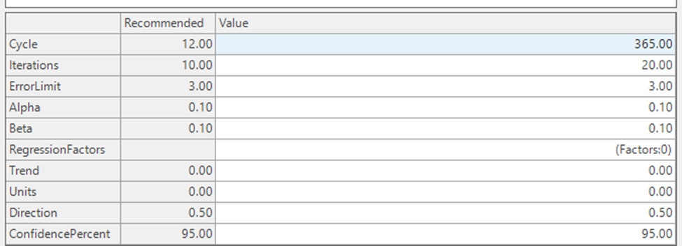
This is based on the Gradient Boosting algorithm with a decision tree method as the week learner. The decision tree algorithm uses the underlying attributes of the data such as time periods as factors. This allows for disaggregation of time date attributes such as day, week, month, quarter and Year. External factors can also be included in addition to the time attributes.

Historically, the Demand for an organization is estimated with one of three methods:

manual estimates,
time series analysis,
or simple causal models.

Each has its limits, and none can harness the deep community intelligence every organization has in any but some ad hoc models. Making use of its smart forecasting technology, an advanced machine learning technique called decision trees, and gradient search from optimization, Arkieva has created demand estimation methods that can unleash community intelligence to improve demand estimation and insight.

Parameters

Cycle: Number of periods in a year.
Iterations: Number of iterations
Error Limit
Alpha: takes values between 0 and 1, this is the learning rate, rate at which residual slices are used to update the forecast
Beta: tracks the direction of the error.
Regression factors: there are factors to control the model. It provides the ability to include Regression Factors as an additional input.

Constant0

Constant0 method is used to force the forecast to 0. Mostly it is used when it has been determined that the item is dead or unforecastable.

This method can be used in cases where a certain product is discontinued and is not required to be forecasted. This method also helps in reinitializing the Statistical forecast as 0.

Period Offset

PeriodOffset Method assumes the current forecast is dependent on a prior period value; for example, demand volumes for each day of the week are the same as the same day in the prior week. So, if offset is set to 7 for a daily data, every day of the week has the same volume as the prior week on the same day (e.g. this Monday would be the same as last week's Monday, and would be the same for each day of the week).

Parameters\ The Offset parameter shifts the data forward by the number of periods set in the Value field.

The Alpha parameter increases or decreases the future volume. If the offset value is 0.1 then it would increase the value by 10%. So, if offset=1 and alpha is 0.1, then it would increase the prior period’s value by 10%. If set to -0.1 then it would decrease the value by 10%. This is used in situations where future volumes are like prior volumes. For example, seasonal data.

Offset Example 1 offset =1; current period is the same as previous period\ In the example below, the offset is set to 1. So, the new value for Dec 17 would be the same as the value for Nov 17, also the value for Jan 18 would be the value for Dec 17.

offset =1; current period is the same as previous period

Offset Example 2 offset =3; current period is than same as 3 periods back\ In the example below, the offset is set to 1. So, the new value for Feb 18 would be the same as the value for Nov 17, also the value for Mar 18 would be the value for Dec 17.

offset =3; current period is than same as 3 periods back

Offset and Alpha Example offset=1, alpha=0.1; current period is 10% more than the previous period**\ This is implemented after the current date. Between Nov 17 and Dec 18, the numbers would the same as example 1, the 20% increase is implemented start from Jan 19. So, Jan 1 is 20% more than Dec 18.

offset=1, alpha=0.1: current period is 10% more than the previous period

R Arima

📘 R Method

R is an open source programming language and environment for statistical computing and graphics. R provides a wide variety of statistical and graphical techniques, and is highly extensible.

For the R methods, we auto-populate the confidence intervals (lower and upper bound).

Arkieva has an Arima forecasting method that handles only non-seasonal models. R Arima extends this function to include seasonal models, event factors, and external (regression) factors. There are two R Arima methods:

R Arima\ In addition to the non-seasonal parameter, seasonal parameters are included to handle seasonality. It is the user’s responsibility to select the right set of parameters for the model.

R Auto Arima\ R Auto Arima (RAutoArima): automatically selects the optimal parameters for the Arima method to generate the best fit. Auto Arima implements Regression factors but not Event Factors. With the exceptions of Regression factors, changes to the parameters included with the interface are never used in the model, the objective was to update the parameters once the optimal values have been determined. The updates to the parameter is yet to be implemented.

R Intermittent

📘 R Method

R is an open source programming language and environment for statistical computing and graphics. R provides a wide variety of statistical and graphical techniques, and is highly extensible.

For the R methods, we auto-populate the confidence intervals (lower and upper bound).

For forecasting sporadic data. If data is not considered sporadic then no forecasting is done.

When selecting R Intermittent methods, except for the select type, all other parameters are determined by the model.

When only a single method is selected, the default run is sequential. On average, this might take a bit longer when an item is selected and has to calculate the performance metric. The data is passed to R one window at a time, depending on the Arkieva Forecast. Errors are handled in Arkieva.

When multiple methods are selected, the data and methods are grouped together and pushed to R for parallel processing. When an item is selected, one item and all window intervals are pushed to R for parallel processing. Most of the forecasting errors are managed in R. If a forecast fails, a result is still returned, and the historical data will be used as fitted and the future forecast will be the average of the historical data. This will prevent all items forecast from failing.

Intermittent Rate\ Applies exponential smoothing to a ratio of the quantity over the duration since the last non-zero quantity.

Intermittent Ratio\ Applies the R Auto Arima method to the transformed cumulative rate and then transforms back to the original form.

Intermittent Regression\ Applies a regression analysis on the cumulative sum of the period.

R Intermittent Croston\ Uses Croston from the forecast package.

R Intermittent Optimal\ Uses Intermittent Multiple Aggregation Prediction Algorithm (IMAPA) from the R package intermittent.

Winter's methods

Winter's is a cyclical method. Cyclical meaning any repeating pattern. For example a business might have a cyclical pattern of 52 weeks that starts in January and ends in December, or a business might have a cyclical pattern of 26 weeks that starts in March, etc.

Winter's Additive\ This method models seasonal data by iteratively fitting a trend to history along with an adjustment for each month. The adjustment is added on each month after the trend is updated. It works best with at least 3 full years of history for estimating the adjustments. Winters additive (along with Winters multiplicative) is more robust than the curve-fitting seasonal methods, but the results will not be as good for smooth, stable series.

Three parameters effect the relative weighting of history in the estimation of the intercept, the trend, and the seasonal adjustments: Alpha affects the intercept, Beta affects the slope, and Gamma affects the seasonal adjustments.

Each of these three parameters can be varied from 0.05 to 0.5 to increase the weighting of recent history during the estimation procedure. At the 0.05 level the three (or more) past years are weighted relatively evenly whereas at the 0.5 level the of effect of the most recent two years is pronounced. The MultiRegWeight and Damping parameters are used only in the case where there is not enough history to estimate the parameters, in which case an ordinary linear regression is used.

Winter's Multiplicative\ This method is the same as Winters additive except that the seasonal adjustments for each month multiplies the current value of the trend line rather than adding to it. This can result in a better forecast when the slope is large. The effects of the parameters are the same as for Winters additive.

Winter's Optimum Additive\ This method uses curve-fitting to attempt to select the values of the parameters alpha, beta, and gamma for the Winters additive method which give the “best” results. The algorithm does not use the given alpha, beta, or gamma parameters. The damping and MultiRegWeight parameters are used only in the case where there is not enough history to run Winters method, in which case a linear regression is used to forecast the series. This method will usually produce a good forecast, but the error criterion is based on fitting a curve to past history, so it doesn’t always have superior predictive ability to the ordinary additive Winters method

The range of values considered for optimization is from 0.05 to 0.6 for all smoothing parameters. Anything more or less was too extreme. The “optimum” values are found by a nonlinear optimization algorithm called Nelder-Mead. It makes very minimal assumptions about the behavior of the objective function. The current algorithm does not need an increment as it picks its own every iteration. It is optimizing the MSE of the forecast vs the history, as that is the standard way that Winters Optimization works.

Winter's Optimum Multiplicative\ This method is the same as Winters optimum additive except the parameters Alpha, Beta and Gamma are chosen to minimize the MSE of the historic forecast.

Single Exponential

Weighted Average formula where the weights decrease exponentially by a factor of (1 – Theta)

Use Theta in the .05 to .30 range. Larger values of Theta make the forecasts more dependent on recent history. Below is a table that shows the weights for ‘k’ time periods back based on a value of Theta. As Theta increases, more weight is assigned to more recent observations, or the weight on the observations further back in history decreases at a more rapid pace.

General formula

This method requires specifying a value of θ which is typically a fraction between 0 and 0.2. This parameter is then used to calculate the forecast as follows.

The above equation can be read as forecast of period t+1 is a weighted sum of actuals from period t to (t-2) plus (1−θ)^3 times forecast of period (t−2). This can be extended recursively till the start of time series data that we have, that is till we have a valid actual sales value.

Now the weights for each history period can be observed to follow a series as θ,θ(1−θ),θ(1−θ)2,θ(1−θ)3,θ(1−θ)2………and so on which is the approximation of exponential series, hence the name exponential smoothing. Note that the standard original exponential formula is y = ab^z.

This would mean the latest actual data has highest weightage and oldest data point has least weightage. In other words the contribution of (1−θ)^n decreases with each time interval. Depending on the value of θ, this can approach 0 very quickly. So by controlling the value of θ we can control what impact of history need to be considered while forecasting.

Arkieva also offers parameterized control over the number of history periods that will be considered during the forecasting process. This parameter is called lag. Based on the above facts, as well as the business conditions, one can decide how far back one would like to go in history when computing the forecast. Then, the effect of observations that are older than this decided number of periods can be ignored. Arkieva utilizes this method of implementation. Therefore, results from Arkieva’s single exponential method are different from the textbook single exponential method, if the lag parameter is less than the number of periods in history (if the lag parameter is less than the number of periods in history, all the data points in history will not be considered while forecasting). One can set lag equal to the number of periods of history to get to the same results as the textbook method.

Arkieva Implementation\ Shown below is a screenshot of where the parameters are set in Arkieva for the single exponential method.

Theta means θ as per the description above
Lag controls how far back the algorithm goes back in the past.
Offset controls where to start the calculation.

The default value is -1. That means that forecast in this period is calculated based on actuals in previous period and prior periods.

If one sets this to 11, then it is interpreted as -1+-11, which is -12. In a setup with monthly periods, this would mean that forecast is being calculated based on what happened exactly 12 months (or 1 year) ago.

This is then normalized such that the weights add up to 1.

From this point, the single exponential smoothing formula works exactly like the weighted averages formula. The only difference is that the weights are derived from the value of θ and lag parameters.

The table below shows how the values of ωn that is (1−θ)^n change as one goes back in time for different values of θ. Higher the θ, faster the value converges to 0. It is worth noting that a value 0 implies that single exponential works just like the moving average method.

📘 We have the following choices:

Simple Period Average always applies equal weights (user does not have to choose the weights).

Weighted Average method where user will define the weights in application.

Use the single exponential method to set the parameter which does calculation and applies the weights.

Straight Line

Another name for Linear Regression.

Unitize

Used as an ‘after’ procedure to put a forecast into unit sizes while preserving the total forecast volume over time

It has two parameters: the unit size and the direction. The procedure will ‘round’ the forecast value to the unit size. The direction is used to determine the fraction of a unit size needed to round up. Any rounding error is added/subtracted to the next period forecast. If the directions are close to zero, the forecast will be “pulled forward”. If it is close to 1, it will be pushed back. The total forecast will always be within one unit of the original forecast.

Units and Direction
ConfidencePercent

Purpose of Unitization\ Any plan data is expressed in time. So, we might have data that expresses planned shipments to customers on a day by day basis based on the current demand projection, or one might have the monthly forecast broken into daily forecast using some simple rules.

These data points might not be in proper increments. For example, the shipments data might need to be in multiples of truck loads if that is how we ship. Forecast data might need to be in multiples of pallet sizes if that is how we sell. However, the input data stream might not follow these rules and we might need to convert these forecasts in multiples of appropriate units.

In Arkieva we call this ‘unitization’.

How do we Unitize?

Any time series data can be unitized using the pr_UN_Lotsize_Netting procedure. This procedure is embedded here:

/****** Object:  StoredProcedure [dbo].[pr_UN_LotSize_Netting]    Script Date: 5/9/2017 4:40:47 AM ******/
SET ANSI_NULLS ON
GO
SET QUOTED_IDENTIFIER ON
GO
/*
    Perform Unitization of Netting data using push/pull logic.
    The @source_tbl and @unit_tbl tables must be name of a netting table or view
    and the name of a unitization table or view, respectively.  The attributes being
    netted upon in @source_tbl must be the same attributes defined for unitization in
    @unit_tbl

    V001.005    JES  03/23/2016  Changes to specs -- esp. output quanity to be in original units ( like LB or KG ), not in Unit_QT ( which is something like batch )
    V001.004    JES  06/25/2015  Rewrite for efficiency
    V001.003    KAM  02/16/2006  Modified the table compatability logic to allow the source table 
                        to be a global temp table
    V001.002    KAM  12/20/2005  Explicitly define owner as dbo for all tables 
                        created with select into
    V001.001    KAM  06/10/2005  Procedure created

        Input:  
            @source_tbl - The source quantities for unitization
                                    It should have following columns
                                    Attr1 (varchar), Attr2 (varchar), Attr3 (varchar), etc., Date_TM(datetime), Net_Forecast_QT (real)
            @unit_tbl   - The table defining unitizations
                                    It should have the following columns (Attrbute columns must match the column list from @source_tbl exactly)
                                    Unit_Idn (Identitiy Inser column) Attr1 (varchar), Attr2 (varchar), Attr3 (varchar), etc., Unit_QT, Direction_Fraction)
                                    Unit_QT is the amount it will be unitized to; it cannot be 0 or negative.
                                    Direction_Fraction is a number between 0 and 1. It controls when the numbers are rounded up.
                                    0 means immidiately, 1 means when the full lot is available, and other numbers are interpreted by the ratio
            @sql_whe    - Where condition to narrow selection of rows from @source_tbl
            @start_dt   - The beginning date to output to target_tbl
            @end_dt     - The ending date to output to target_tbl

        Output:
            @target_tbl - The table to write out the unitized quantities
*/
-----------------------------------------------------------------------------------------------------------------------------------------------------------------------------   ----|

ALTER   procedure [dbo].[pr_UN_LotSize_Netting]
            @source_tbl         sysname,
            @target_tbl         sysname,
            @unit_tbl           sysname, --         = 'bt_UN_Standard_Units',
            @sql_whe            varchar(4000)   = NULL,
            @start_dt_tx        varchar(100)    = NULL,
            @end_dt_tx          varchar(100)    = NULL

AS

declare
            @att_lst            nvarchar(4000),
            @cmd                nvarchar(4000),
            @join               nvarchar(4000),
            @row_cnt            int,
            @cal_cnt            int,
            @cal_idn            int,

            @message            nvarchar(max),
            @proc_name          sysname,
            @proc_ver           nvarchar(10)

SET NOCOUNT ON

--==============================================
SET         @proc_name      = OBJECT_NAME( @@PROCID )
SET         @proc_ver       = '001.005'
SET         @message        = 'Begin procedure "' + @proc_name + '" V' + @proc_ver + convert(char(30),Current_Timestamp,120)
EXEC        dbo.PrsLogMessage @message, @proc_name, 0
--==============================================

set nocount on

--????? 1 ????? Verify the comptibility between the source table and the unitization table ?????
exec    PrsDropObject #c
create table #c ( column_name varchar(200) )

set     @cmd    = 'insert into #c'
    + ' select column_name from ' + case when left(@source_tbl, 2) = '##' then 'tempdb.' else '' end + 'information_schema.columns where table_name = ''' + @source_tbl + '''' 
    + ' and column_name not in (''Date_TM'', ''Net_Forecast_QT'')'
    + ' and column_name not in ('
    + ' select column_name from ' + case when left(@unit_tbl, 2) = '##' then 'tempdb.' else '' end + 'information_schema.columns'
    + ' where table_name = ''' + @unit_tbl + ''''
    + ' and column_name not in (''Unit_Idn'', ''Unit_QT'', ''Direction_Fraction''))' 

exec    ( @cmd )

set @cmd    = 'insert into #c' 
    + ' select column_name from ' + case when left(@unit_tbl, 2) = '##' then 'tempdb.' else '' end + 'information_schema.columns where table_name = ''' + @unit_tbl + '''' 
    + ' and column_name not in (''Unit_Idn'', ''Unit_QT'', ''Direction_Fraction'')'
    + ' and column_name not in ('
    + ' select column_name from ' + case when left(@source_tbl, 2) = '##' then 'tempdb.' else '' end + 'information_schema.columns'
    + ' where table_name = ''' + @source_tbl + ''''
    + ' and column_name not in (''Date_TM'', ''Net_Forecast_QT''))'
exec    ( @cmd )

if  exists( select * from #c )  begin
    raiserror('Source Table and Unitization Table incompatible', 16, 1)
    return  ( -1 )
end

--????? 2 ????? Prepare for join between source table and unitization table ?????
set @att_lst    = ''
set @join       = ''
select  @att_lst    = @att_lst + 'SRC.[' + column_name + '],',
    @join       = @join + 'SRC.[' + column_name + '] = U.[' + column_name + '] and '
    from    information_schema.columns
    where   table_name  = @unit_tbl
    and column_name not in ('Unit_Idn', 'Unit_QT', 'Direction_Fraction')
    order by    ordinal_position
set @att_lst    = left( @att_lst    , len( @att_lst ) - 1 )     -- remove the trailing comma
set @join       = left( @join       , len( @join    ) - 4 )     -- remove the trailing ' and '

exec        PrsDropObject 'zt_NE_TMP_Calendar'
create      table dbo.zt_NE_TMP_Calendar ( Cal_Idn int not null, Date_TM datetime not null )

--????? 3 ????? create zt_NE_TMP_Calendar ?????
exec        PrsDropObject '#cal'
create      table #cal( Cal_Idn int identity, Date_TM datetime, Tuple_Cnt int )
set         @cmd =  '   insert #cal ( Date_TM, Tuple_Cnt )
                        select SRC.Date_TM, count(*)
                        from [' + @source_tbl   + '] SRC'
                    +   case when @start_dt_tx is null then '' else ' where SRC.Date_TM >= ''' + @start_dt_tx + '''' end 
                    + ' group by SRC.Date_TM
                        order by SRC.Date_TM'

exec    (   @cmd )

insert      zt_NE_TMP_Calendar ( Cal_Idn, Date_TM )
select      Cal_Idn, Date_TM
from        #cal

/*          removed 23-Mar-2016 Sandberg
            --_____ assume every Unit_Idn has the same set of dates _____
set         @cmd = 'insert zt_NE_TMP_Calendar'
                + ' select SRC.Date_TM'
                + ' from [' + @source_tbl   + '] SRC'
                + ' join [' + @unit_tbl     + '] U on ' + @join
                + ' where Unit_Idn = 1'
                + ' order by SRC.Date_TM'

exec    (   @cmd )
*/

set         @cal_cnt = [dbo].fn_Row_Cnt ( 'zt_NE_TMP_Calendar' )
--exec      pr_Log_Row_Cnt 'zt_NE_TMP_Calendar', @cal_cnt, @@procid

--????? 4 ????? create zt_NE_TMP_Input ?????
exec        PrsDropObject 'zt_NE_TMP_Input'
create      table dbo.zt_NE_TMP_Input( Unit_Idn int not null, Cal_Idn int not null, Fcs_QT float not null, Fcs_Adj_QT float not null, Dir_Fra float not null )

set         @cmd    = 'insert into zt_NE_TMP_Input'
                + ' select  U.Unit_Idn
                        ,   C.Cal_Idn
                        ,   SRC.Net_Forecast_QT / cast( U.Unit_QT as float )
                        ,   SRC.Net_Forecast_QT / cast( U.Unit_QT as float )
                        ,   U.Direction_Fraction'
                + ' from [' + @source_tbl   + ']    SRC'
                + ' join [' + @unit_tbl     + ']    U on ' + @join
                + ' join zt_NE_TMP_Calendar         C on SRC.Date_TM = C.Date_TM'

if          @sql_whe is not null set @cmd = @cmd + ' where ' + @sql_whe 

set         @cmd    = @cmd +  ' order by U.unit_idn, C.Cal_Idn'

exec    (   @cmd )

set         @row_cnt = [dbo].fn_Row_Cnt ( 'zt_NE_TMP_Input' )
--exec      pr_Log_Row_Cnt 'zt_NE_TMP_Input', @row_cnt, @@procid

create      unique clustered index zt_NE_TMP_Input_IX on zt_NE_TMP_Input ( Cal_Idn, Unit_Idn )

--????? 5 ????? loop through time periods ?????
exec        PrsDropObject 'zt_NE_TMP_Output'
create      table dbo.zt_NE_TMP_Output( Unit_Idn int not null, Cal_Idn int not null, Fcs_QT float not null, Fcs_Adj_QT float not null, Fcs_Uni_QT float not null )
create      unique clustered index zt_NE_TMP_Output_IX on zt_NE_TMP_Output ( Cal_Idn, Unit_Idn )

set         @cal_idn = 0 while @cal_idn < @cal_cnt begin set @cal_idn = @cal_idn + 1

            insert      zt_NE_TMP_Output
            select      Unit_Idn
                    ,   Cal_Idn
                    ,   Fcs_QT
                    ,   Fcs_Adj_QT
                    ,   case when Fcs_Adj_QT - floor( Fcs_Adj_QT ) > Dir_Fra then floor( Fcs_Adj_QT ) + 1 else floor( Fcs_Adj_QT ) end
            from        zt_NE_TMP_Input
            where       Cal_Idn = @cal_idn
            order by    Unit_Idn

            update      zt_NE_TMP_Input
            set         Fcs_Adj_QT = I.Fcs_Adj_QT - O.Fcs_Uni_QT + O.Fcs_Adj_QT
            from        zt_NE_TMP_Input     I
            join        zt_NE_TMP_Output    O on I.Unit_Idn = O.Unit_Idn
            where       I.Cal_Idn = @cal_idn + 1
             and        O.Cal_Idn = @cal_idn

            end

--????? 6 ????? create @target_tbl ?????
exec        prsDropObject @target_tbl

set         @cmd = ' select ' + @att_lst + ', C.Date_TM, O.Fcs_Uni_QT * U.Unit_QT ''Net_Forecast_QT'', O.Fcs_Uni_QT, U.Unit_QT'
                + ' into dbo.[' + @target_tbl   + ']'
                + ' from [' + @source_tbl   + ']    SRC'
                + ' join [' + @unit_tbl     + ']    U on ' + @join
                + ' join zt_NE_TMP_Calendar         C on SRC.Date_TM = C.Date_TM'
                + ' join zt_NE_TMP_Output           O on U.Unit_Idn = O.Unit_Idn and C.Cal_Idn = O.Cal_Idn'
                + ' where O.Fcs_Uni_QT != 0'

if          @sql_whe        is not null set @cmd = @cmd + ' and ' + @sql_whe
if          @start_dt_tx    is not null set @cmd = @cmd + ' and SRC.Date_TM >= ''' + @start_dt_tx + ''''
if          @end_dt_tx      is not null set @cmd = @cmd + ' and SRC.Date_TM <= ''' + @end_dt_tx + ''''

exec    (   @cmd )

--==============================================
END_PROCEDURE:
SET         @message =  'End   procedure "' + @proc_name + '" V' + @proc_ver + convert(char(30),Current_Timestamp,120)
EXEC        dbo.PrsLogMessage @message, @proc_name, 0

RETURN (0)

The input time series is typically linear in nature; i.e. it does not represent truck loads, or rail car loads, or Each-es, or any such units that actual shipments/sales might take place in. For this reason, there is often a need for unitizing or lot-sizing the continuous (or smooth or linear) input (or forecast or plan). This is done through the pr_UN_Lotsize_Netting procedure.

This procedure has 6 parameters as shown in Table 1 below:

1. Parameter Name: @source_tbl\ The name of the SQL table that has the input data.

It should have following columns:

Attribute 1 (varchar)
Attribute 2 (varchar)
Attribute 3 (varchar)\ etc.
Date_TM (datetime)
Net_Forecast_QT (real)

Net_Forecast_QT is what will be unitized or lot sized.

2. Parameter Name: @unit_tbl\ Table that has the factors for lot sizing.

It should have the following columns (Attribute columns must match the column list from @source_tbl above exactly):

Unit_Idn (Identitiy Insert column)
Attr1 (varchar)
Attr2 (varchar)
Attr3 (varchar)\ etc.
Unit_QT (Integer): (Lot Size; it cannot be 0 or negative)
Direction_Fraction (real): This is a number between 0 and 1. It controls when the numbers are rounded up. Values are rounded up to the next multiple of Unit_QT if the remainder (as a fraction of Unit_QT) exceeds the Direction_Fraction.
If Direction_Fraction equals 0, remainders are always rounded up (PULL).
If Direction_Fraction equals 1, remainders are always rounded down (PUSH).
Other numbers are interpreted by the ratio or percentage

3. Parameter Name: @target_tbl\ The name of the SQL table where the output will go. If the table does not exist, it will be created by the procedure. If it does exist, then the procedure will not delete any records from it. Please take note.

The output will have all the attributes from @source_tbl:

Attr1 (varchar)
Attr2 (varchar)
Attr3 (varchar)\ etc.
Date_TM (datetime)
Net_Forecast_QT (real): This is the lot sized quantity based on criteria defined in @unit_tbl above.
Fcs_Uni_QT (integer): Number of lots or units
Unit_QT (Integer): Lot Size from table @Unit_tbl above

4. Parameter Name: @sql_whe\ A where clause to filter out (or in) only those records that one wants to process from @source_tbl.

5. Parameter Name: @start_dt_tx\ Start Date of the processing before which the data will be ignored from @source_tbl.

6. Parameter Name: @end_dt_tx\ End Date of the processing after which the data will be ignored from @source_tbl.

The total forecast across periods does not change because of this procedure. Therefore, the last period often gets a quantity that is not a multiple of the Units Parameter.\ The Following table shows an example of forecast being unitized with ‘Units’ parameter set to 10, and different values of the ‘Round’ parameter.

Table 2: Unitization Results

This same code can be used to convert fractional numbers to integers.

Table 3: Converting Fractional forecast to integers

Unitization to Weekdays\ Same code can be used to unitize to different days of the week. See example below. In most instances, this is an overkill.

Table 4: Unitization Results

Example Screenshots:

Input Table (@source_tbl)

Factors Table (@unit_tbl)

Output Table (@target_tbl)

How to call the procedure:

EXEC [dbo].[pr_UN_LotSize_Netting]
@source_tbl = 'zvw_Z_FG_SalesPlan_Unitization_Input',
@target_tbl = 'ztb_FG_SalesPlan_Unitization_Output',
@unit_tbl   = 'zvw_Z_FG_SalesPlan_Unitization_Factors',
@Start_dt_Tx    = '2017-05-08'

Unitization to particular days of week\ In certain situations, the linear forecast needs to be lot size or unitized to a particular day(s) of the week. For example, we might want to lot size the forecast to coincide with days of the week when a boat is scheduled to leave the dock. To enable this, the procedure below is helpful: Please note that the procedure below is only lightly tested. Since the procedure above can be replicated by this procedure, we should test this and use this one.

/****** Object:  StoredProcedure [dbo].[pr_UN_LotSize_Netting_DOW]    Script Date: 5/9/2017 5:10:34 AM ******/
SET ANSI_NULLS ON
GO
SET QUOTED_IDENTIFIER ON
GO
/*
    Perform Unitization of Netting data using push/pull logic.
    The @source_tbl and @unit_tbl tables must be name of a netting table or view
    and the name of a unitization table or view, respectively.  The attributes being
    netted upon in @source_tbl must be the same attributes defined for unitization in
    @unit_tbl

    V001.005    JES  10/17/2015  Add day-of-week processing
    V001.004    JES  06/25/2015  Rewrite for efficiency
    V001.003    KAM  02/16/2006  Modified the table compatability logic to allow the source table 
                        to be a global temp table
    V001.002    KAM  12/20/2005  Explicitly define owner as dbo for all tables 
                        created with select into
    V001.001    KAM  06/10/2005  Procedure created

        Input:  
            @source_tbl - The source quantities for unitization
                                    It should have following columns
                                    Attr1 (varchar), Attr2 (varchar), Attr3 (varchar), etc., Date_TM(datetime), Net_Forecast_QT (real)
            @unit_tbl   - The table defining unitizations
                                    It should have the following columns (Attrbute columns must match the column list from @source_tbl exactly)
                                    Unit_Idn (Identitiy Inser column) Attr1 (varchar), Attr2 (varchar), Attr3 (varchar), etc., Unit_QT, Direction_Fraction)
                                    Unit_QT is the amount it will be unitized to; it cannot be 0 or negative.
                                    Direction_Fraction is a number between 0 and 1. It controls when the numbers are rounded up.
                                    0 means immidiately, 1 means when the full lot is available, and other numbers are interpreted by the ratio
            @sql_whe    - Where condition to narrow selection of rows from @source_tbl
            @start_dt   - The beginning date to output to target_tbl
            @end_dt     - The ending date to output to target_tbl

        Output:
            @target_tbl - The table towrite out the unitized quantities
*/
-----------------------------------------------------------------------------------------------------------------------------------------------------------------------------   ----|

ALTER   procedure [dbo].[pr_UN_LotSize_Netting_DOW]
            @source_tbl         sysname,
            @target_tbl         sysname,
            @unit_tbl           sysname         = 'bt_UN_Standard_Units',
            @sql_whe            varchar(4000)   = NULL,
            @start_dt_tx        varchar(100)    = NULL,
            @end_dt_tx          varchar(100)    = NULL,
            @dow_list           varchar(100)    = 'Sun,Mon,Tue,Wed,Thu,Fri,Sat'

AS

declare
            @att_lst            nvarchar(4000),
            @cmd                nvarchar(4000),
            @join               nvarchar(4000),
            @row_cnt            int,
            @cal_cnt            int,
            @cal_idn            int,
            @dow                char(3),
            @dow_list_YN        char(1),

            @message            nvarchar(max),
            @proc_name          sysname,
            @proc_ver           nvarchar(10)

SET NOCOUNT ON

--==============================================
SET         @proc_name      = OBJECT_NAME( @@PROCID )
SET         @proc_ver       = '001.005'
SET         @message        = 'Begin procedure "' + @proc_name + '" V' + @proc_ver + convert(char(30),Current_Timestamp,120)
EXEC        dbo.PrsLogMessage @message, @proc_name, 0
--==============================================

set nocount on

--????? 1 ????? Verify the comptibility between the source table and the unitization table ?????
exec    PrsDropObject #c
create table #c ( column_name varchar(200) )

set     @cmd    = 'insert into #c'
    + ' select column_name from ' + case when left(@source_tbl, 2) = '##' then 'tempdb.' else '' end + 'information_schema.columns where table_name = ''' + @source_tbl + '''' 
    + ' and column_name not in (''Date_TM'', ''Net_Forecast_QT'')'
    + ' and column_name not in ('
    + ' select column_name from ' + case when left(@unit_tbl, 2) = '##' then 'tempdb.' else '' end + 'information_schema.columns'
    + ' where table_name = ''' + @unit_tbl + ''''
    + ' and column_name not in (''Unit_Idn'', ''Unit_QT'', ''Direction_Fraction''))' 

exec    ( @cmd )

set @cmd    = 'insert into #c' 
    + ' select column_name from ' + case when left(@unit_tbl, 2) = '##' then 'tempdb.' else '' end + 'information_schema.columns where table_name = ''' + @unit_tbl + '''' 
    + ' and column_name not in (''Unit_Idn'', ''Unit_QT'', ''Direction_Fraction'')'
    + ' and column_name not in ('
    + ' select column_name from ' + case when left(@source_tbl, 2) = '##' then 'tempdb.' else '' end + 'information_schema.columns'
    + ' where table_name = ''' + @source_tbl + ''''
    + ' and column_name not in (''Date_TM'', ''Net_Forecast_QT''))'
exec    ( @cmd )

if  exists( select * from #c )  begin
    raiserror('Source Table and Unitization Table incompatible', 16, 1)
    return  ( -1 )
end

--????? 2 ????? Prepare for join between source table and unitization table ?????
set @att_lst    = ''
set @join       = ''
select  @att_lst    = @att_lst + 'SRC.[' + column_name + '],',
    @join       = @join + 'SRC.[' + column_name + '] = U.[' + column_name + '] and '
    from    information_schema.columns
    where   table_name  = @unit_tbl
    and column_name not in ('Unit_Idn', 'Unit_QT', 'Direction_Fraction')
    order by    ordinal_position
set @att_lst    = left( @att_lst, len( @att_lst ) - 1 )     -- remove the trailing comma
set @join       = left( @join, len( @join ) - 4 )       -- remove the trailing ' and '

exec        PrsDropObject 'zt_NE_TMP_Calendar'
create      table zt_NE_TMP_Calendar ( Cal_Idn int identity not null, Date_TM datetime not null )

--????? 3 ????? create zt_NE_TMP_Calendar ?????
            --_____ assume every Unit_Idn has the same set of dates _____
set         @cmd = 'insert zt_NE_TMP_Calendar'
                + ' select SRC.Date_TM'
                + ' from [' + @source_tbl   + '] SRC'
                + ' join [' + @unit_tbl     + '] U on ' + @join
                + ' where Unit_Idn = 1'
                + ' order by SRC.Date_TM'

exec    (   @cmd )

set         @cal_cnt = [dbo].fn_Row_Cnt ( 'zt_NE_TMP_Calendar' )
exec        pr_Log_Row_Cnt 'zt_NE_TMP_Calendar', @cal_cnt, @@procid

--????? 4 ????? create zt_NE_TMP_Input ?????
exec        PrsDropObject 'zt_NE_TMP_Input'
create      table zt_NE_TMP_Input( Unit_Idn int not null, Cal_Idn int not null, Fcs_QT float not null, Fcs_Adj_QT float not null, Dir_Fra float not null )

set         @cmd    = 'insert into zt_NE_TMP_Input'
                + ' select  U.Unit_Idn
                        ,   C.Cal_Idn
                        ,   SRC.Net_Forecast_QT / cast( U.Unit_QT as float )
                        ,   SRC.Net_Forecast_QT / cast( U.Unit_QT as float )
                        ,   U.Direction_Fraction'
                + ' from [' + @source_tbl   + ']    SRC'
                + ' join [' + @unit_tbl     + ']    U on ' + @join
                + ' join zt_NE_TMP_Calendar         C on SRC.Date_TM = C.Date_TM'

if          @sql_whe is not null set @cmd = @cmd + ' where ' + @sql_whe 

set         @cmd    = @cmd +  ' order by U.unit_idn, C.Cal_Idn'

exec    (   @cmd )

set         @row_cnt = [dbo].fn_Row_Cnt ( 'zt_NE_TMP_Input' )
exec        pr_Log_Row_Cnt 'zt_NE_TMP_Input', @row_cnt, @@procid

create      unique clustered index zt_NE_TMP_Input_IX on zt_NE_TMP_Input ( Cal_Idn, Unit_Idn )

--????? 5 ????? loop through time periods ?????
exec        PrsDropObject 'zt_NE_TMP_Output'
create      table zt_NE_TMP_Output( Unit_Idn int not null, Cal_Idn int not null, Fcs_QT float not null, Fcs_Adj_QT float not null, Fcs_Uni_QT float not null )
create      unique clustered index zt_NE_TMP_Output_IX on zt_NE_TMP_Output ( Cal_Idn, Unit_Idn )

set         @cal_idn = 0 while @cal_idn < @cal_cnt begin set @cal_idn = @cal_idn + 1

            select      @dow = left( datename( DW, Date_TM ), 3 ) from zt_NE_Tmp_Calendar where Cal_Idn = @cal_idn
            set         @dow_list_YN = case when charindex( @dow, @dow_list ) > 0 then 'Y' else 'N' end
            print       @dow + ' ' + @dow_list_YN

            insert      zt_NE_TMP_Output
            select      Unit_Idn
                    ,   Cal_Idn
                    ,   Fcs_QT
                    ,   Fcs_Adj_QT
                    ,   case when @dow_list_YN = 'N'
                            then 0
                            else case when Fcs_Adj_QT - floor( Fcs_Adj_QT ) > Dir_Fra
                                    then floor( Fcs_Adj_QT ) + 1
                                    else floor( Fcs_Adj_QT )
                                    end
                            end
            from        zt_NE_TMP_Input
            where       Cal_Idn = @cal_idn
            order by    Unit_Idn

            update      zt_NE_TMP_Input
            set         Fcs_Adj_QT = I.Fcs_Adj_QT - O.Fcs_Uni_QT + O.Fcs_Adj_QT
            from        zt_NE_TMP_Input     I
            join        zt_NE_TMP_Output    O on I.Unit_Idn = O.Unit_Idn
            where       I.Cal_Idn = @cal_idn + 1
             and        O.Cal_Idn = @cal_idn

            end


--????? 6 ????? create @target_tbl ?????
exec        prsDropObject @target_tbl

set         @cmd = ' select ' + @att_lst + ', C.Date_TM, U.Unit_QT*O.Fcs_Uni_QT ''Net_Forecast_QT'''
                + ' into [' + @target_tbl   + ']'
                + ' from [' + @source_tbl   + ']    SRC'
                + ' join [' + @unit_tbl     + ']    U on ' + @join
                + ' join zt_NE_TMP_Calendar         C on SRC.Date_TM = C.Date_TM'
                + ' join zt_NE_TMP_Output           O on U.Unit_Idn = O.Unit_Idn and C.Cal_Idn = O.Cal_Idn'
                + ' where O.Fcs_Uni_QT != 0'

if          @sql_whe        is not null set @cmd = @cmd + ' and ' + @sql_whe
if          @start_dt_tx    is not null set @cmd = @cmd + ' and SRC.Date_TM >= ''' + @start_dt_tx + ''''
if          @end_dt_tx      is not null set @cmd = @cmd + ' and SRC.Date_TM <= ''' + @end_dt_tx + ''''

exec    (   @cmd )

--==============================================
END_PROCEDURE:
SET         @message =  'End   procedure "' + @proc_name + '" V' + @proc_ver + convert(char(30),Current_Timestamp,120)
EXEC        dbo.PrsLogMessage @message, @proc_name, 0

RETURN (0)

This procedure is almost identical with the procedure above with one difference: It has one extra parameter. It takes as parameter a comma delimited list of days of week when lot sizing is allowed. The extra parameter is like this:

@dow_list   varchar(100)    = 'Sun,Mon,Tue,Wed,Thu,Fri,Sat'

The default is that shipments are allowed on all days. But, if this parameter is passed as 'Tue,Thu', then this procedure will lot size everything to only Tuesday and Thursday. But, as noted, this is not fully tested.

Weights

This method works the same way as single exponential smoothing, except that the successive weights moving backwards in time can be defined more explicitly. For example, single exponential smoothing with theta = 0.05 has weights 1, 0.95, 0.90, 0.86, 0.81, 0.77, 0.74, etc. With the Weights method, you could instead define weights 1, 0.95, 0.90, 0.85, 0.80, 0.75.0.70, for example. The method isn’t hard to use, but most often the canned weights available with exponential smoothing provide a sufficient range of possibilities.

Optimize

Select Weights from the Forecast Method dropdown to see the Forecast Score Weighted Summary average.

Moving Average

Simple Moving Average, Weighted Moving Average, and Single Exponential Smoothing are Moving Average Methods that always give an average forecast, i.e. a flat line. This is because once the History ends, it only has the last forecast available which is then published to future periods.

Simple Moving Average Method\ The Moving Average Method only takes the average of the historical data, it does not consider any pattern. If there is a data set of 10, 18, and 24, then the 3 Period Moving Average is 17.33. If there is a data set of 24, 18, and 10, then the 3 Period Moving Average is still 17.33. The Simple Moving Average method does not consider the data has a declining trend. We are assigning equal weights to all the periods in a Simple Moving Average method.

Simple Moving Period Average always applies equal weights (user does not have to choose weights).

Example 1: If value of period is set\ If the forecast is generated using an Average method with Period set to 3 , then the forecast is calculated by taking the average of the last 3 periods history.

If the the period >= Current Period, it will hold the last calculated forecast value.

Current Period: 6/27/2020
Period: 3
Calculation: Forecast generated for 6/24/2020 is 52 which is the average of 53, 71 and 33. Forecast generated for period greater than and equal to 6/27/2020 is 66 which is the average of 52, 67 and 78.

Hence the period average method always generates a flat line forecast into the future whereas forecast is variable in the past periods.

Example 2: If value of period is set\ If the forecast is generated using the Average method with Period set to 1 , then the forecast calculated is equal to the last historical period value.

Example 1: If values for period and offset is set

If the forecast is generated using the Average method with Period set to 1 and Offset set to 6, then the forecast is equal to the history from 7 periods ago (go back by default 1 period).

Current Period: 6/27/2020
Period: 1
Offset: 6
Calculation: Forecast generated for 6/27/2020 is 50 which is the history as on 6/20/2020. Forecast generated for 6/28/2020 is 53 which is the history as on 6/21/2020 and So on. Forecast generated for period greater than and equal to 7/3/2020 is 78 which is holding the history as on 6/26/2020.

Example 2: If values for period and offset is set

If the forecast is generated using Average method with Period set to 3 and Offset set to 5, then go back 5 periods; forecast is calculated by taking the average of 3 periods history.

Current Period: 6/27/2020
Period: 3
Offset: 5
Calculation: Forecast generated for 6/27/2020 is 56 which is the average of 66, 50 and 53. Forecast generated for 6/28/2020 is 58 which is the average of 50, 53 and 71 and so on. Forecast generated for period greater than and equal to 7/2/2020 is 66 which is the average of 52, 67 and 78.

📘 Note

For weekly cycle, offset is 6 (if period is set to 1)

For monthly cycle, offset is 11 (If period is set to 1)

Offset method is the simplest way to forecast seasonality.

Weighted Moving Average Method\ Instead of equally weighing all periods, Weighted Moving Average assigns weights to every period based on recency. Generally, the more recent the period the heavier the weight. Use Weighted Moving Average to define weights.

Here we do period average again but instead of weighing them equally we put weights on them

Example 1\ If the forecast is generated using the Weight method with Number of weights set to 3, where:

Weights1 = 0.5 (for the period which is 1 period prior put weight of 50%)
Weights2 = 0.4 (for the period which is 2 period prior put weight of 40%)
Weights3 = 0.1 (for the period which is 3 period prior put weight of 10%)

Then it will calculate the weighted 3 period average of the last 3 periods of history.

Current Period: 6/27/2020
Calculation: Forecast generated for 6/27/2020 is 71 which is the weighted average of 52, 67 and 78.\ I.e. 78_0.5 = 39, 67_0.4 = 26.8, 52*0.1=5.2; then calculate the SUM = 39+ 26.8+ 5.2 = 71.

📘 Note

To assign more weights to more recent periods use the weighted Average method.

To calculate the weighted average of 7 periods, change the Number of Weights = 7 and set percentage weights from weight 1 till weight 7.

Single Exponential Smoothing\ Instead of manually assigning weights to every single period we can provide a factor called theta to the engine, and the engine will assign the weights. Uses parameters to apply the weights to past periods. Use the single exponential smoothing method to set the parameter for calculation and applying weights.

Single Exponential Smoothing method is suitable for a data set that has no tend and seasonality. This method uses parameter Theta to apply the weights to past periods. Since the method is valid for data set without any trend or seasonality, the underlying assumption is that forecast for a period is forecast for previous period +_delta. One way of defining this delta is a weighted factor of forecast deviation (Actual - Forecast) observed in last period.

Forecast in any period t(S_t) is based on the forecast in the previous period (S_t-1) and forecast deviation from the previous period. Forecast deviation from previous period (X_t-1 - S_t-1), where X_t-1 is the actual sales in previous period.

S_t = S_t + 0(X_t-1 - S_t-1)

Rearranging the variables we get the formula as

S_t = (1 - 0)S_t + 0X_t-1

The same formula can be used to derive forecast for next period (t + 1) as

S_t+1 = (1 - 0)S_t + 0X_t

Substituting for S_t, we get

S_t+1 = (1 - 0)((1 - 0)S_t-1 + 0X_t-1) + 0X_t\ S_t+1 = (1 - 0)^2 S_t-1 + 0(1 - 0) X_t-1 + 0X_t\ .\ .\ .\ .\ S_t+1 = (1 - 0)^3 S_t-2 + 0(1 - 0)^2 X_t-2 + 0(1 - 0) X_t-1 + 0X_t

The above equation can be read as forecast of period t+1 is a weighted sum of actuals from period t to )t-2) plus (1 - 0)^3 times forecast of period (t - 2). This can be extracted recursively until the start of time series data that we, that is until we have a valid actual sales value. Now the weights of each history period can be observed to follow a series as

0,0 (1 - 0), 0(1 - 0)^2, 0(1 - 0)^3, 0(1 - 0)^2 ......... and so on which is the approximation of exponential series, hence the name exponential smoothing. Note that the standard original exponential formula is y=ab^z.

Rearranging the equation

S_t+1 = θX_t + θ(1−θ)X_t−1 + θ(1−θ)^2 X_t−2 + (1−θ)^3 S_t−2

It should be noted that for a positive value of 0 \< 1 the weights decreases exponentially. For example for value of 0 = 0.2

θ θ(1−θ) θ(1−θ)2 θ(1−θ)3 θ(1−θ)4 θ(1−θ)5 θ(1−θ)6

Example\ If the parameter is set to 0.1 then immediately preceding period will get full weight.

Period which is 2 periods prior will get 90%
Period which is 3 periods prior will get 82%

According to which weights will be applied, 36%, 33% and 30%, respectively.

If the parameter is set to 0.2 then the immediately preceding period will get full weight.

Period which is 2 periods prior will get 83%
Period which is 3 periods prior will get 69%

The bigger the parameter value the faster the weight decreases.

Cyclical methods

Cyclical means any repeating pattern. For example a business might have a cyclical pattern of 52 weeks that starts in January and ends in December, or a business might have a cyclical pattern of 26 weeks that starts in March, etc.

For Monthly Forecasting, Cycle parameter should be set as 12
For Weekly Forecasting, Cycle parameter should be set as 12
For Daily Forecasting, Cycle parameter should be set as 7

All cyclical methods look for the cycle and trend. They require damping for that reason.

Fourier method does not have a cycle parameter. This method tries to figure out the cycle on its own.

Seasonal

The Seasonal method is a regression method fitting a linear trend (as with linear regression) along with sine and cosine curves that allow nearly any seasonal departure from the trend to be fit. This method is best for a series with a long term stable trend. For less consistent series, some of the other seasonal methods will probably be better.

Parameters:

Cycle
MultiRegWeight
DampingFactor
Units and Direction
ConfidencePercent

Robust Seasonal

Like Seasonal, this method fits a trend along with sine and cosine curves. This method uses linear programming to fit a seasonal series in a way that — compared to the regular seasonal method — is less likely to be thrown off by noisy values that depart from the trend or seasonality.

The two penalty parameters refer to additional effects that the method is capable of estimating. The method is capable of detecting a “level shift” where there is a one-time increase of decrease in the overall level of the series. It can also detect if there is a single month where the series has a seasonal adjustment that departs from the sine and cosine curves that the model is trying to fit.

If the “penalty” for one of these effects is high — at the default value of 2.0 — then it will not affect the result. If the penalty is reduced to 1.5, the given effect can come into play. In order for the penalties to be lowered, there should be at least several years of history in order to estimate the underlying trend and seasonality.

Parameters:

Cycle
ShiftPenalty
PeriodPenalty
DampingFactor
Units and Direction
ConfidencePercent

Lewandowski\ Lewandowski is an iterative method to forecast trends and seasonality.

Cycle = number of periods per year. Parameters alpha, beta, gamma, choose values close to 0. Larger values mean more influence for recent observations. Damp 1 = no damping of trends; choose values less than 1 to damp trends. Smooth: 1 = smooth parameters for weekly data, 0 = do not smooth.

Parameters:

Cycle
Alpha
Beta
Gamma
DampingFactor
Units and Direction
ConfidencePercent

Arima\ The Arima method is a system of “engines” that can produce curves to fit and forecast a time series. Each choice of the three parameters ArimaP, ArimaD, and ArimaQ (or just P ,D, and Q) defines a different engine that may be useful in forecasting the series. Each of these parameters should be an integer, satisfying 0 \<= P \<= 2, 0\<= D \<= 1, and 0 \<= Q \<= 2.

The engines having D= 0 produce series with no trend; those with D = 1 produce trends.

Parameters P and Q don’t have a natural interpretation in terms of the properties of the series. A simple way to select a variety of engines is to select P and Q satisfying P+Q = 2, so that (P,Q) takes the values (2,0), (0,2), and (1,1).

Each engine (i.e., each choice of P, D, and Q) is a model with its own parameters (not shown here) that are selected to best fit the historical data. Several of these models can be pitted against each other to see which is most successful in predicting the future.

Cycle
Arima
Units and Direction
ConfidencePercent

Fourier\ Fourier is a special cyclical method which tries to find the cycle on its own. Fourier is a curve-fitting techniques are used to fit a combination of sine and cosine curves to the series. For very stable series with no trend, this can provide the best fit, but in most other situations one of the seasonal methods should work better.

Intermittence methods

Intermittent data is data where it will have lots of zeros in the middle ( I.e. 50% or more observations are zeros after ignoring leading zeros).

Below is the way to calculate and know if series is intermittent.


3 Years of History	36
Leading zeros?	13
Periods to consider	23
Non zero observations	11
% Non zero observations (Non zero observations/Periods to consider)	39%
% Zero observations (Zero observations/Periods to consider)	61%
If % Zero Observations > 50%, the series is intermittent.

📘 Note

If the series is intermittent as well as seasonal, you will need to apply both types of methods, i.e. seasonal methods and methods for intermittence.

Sporadic\ The Sporadic method attempts to predict sporadic or intermittent time series. Sporadic tries to predict the size of the peaks, and the gaps in the peaks.

This method looks for a pattern where most values in the series are 0, with positive values occurring at nearly regular intervals. If the series does not show such a pattern, it is forecast via single exponential smoothing, using the parameters lag and theta. On the other hand, if a sporadic pattern can be detected, the pattern is projected into the future by applying exponential smoothing to the individual positive values.

Parameters:

NumberOfWeights
Lag
Alpha
Theta
MaxPctPos
SporadicOption
Units and Direction
ConfidencePercent

Croston\ The Croston method attempts to predict sporadic or intermittent time series. Croston tries to predict the size of the peaks, and the gaps in the peaks.

Croston deals with the same situations as the Sporadic method, except that an improved algorithm is used to generate the forecast values for future events.\ This algorithm works in two different ways:

By default – when the Syntetos-Boylen parameter is set to 1 – it uses the “Syntetos-Boylan” correction.
With this parameter kept at 1, the method will usually produce better results than the Sporadic method.

Parameters:

NumberOfWeights
Lag
Alpha
Theta
Cycle
Syntetos-Boylen
Units and Direction
ConfidencePercent

Intermittent Rate\ Applies exponential smoothing to a ratio of the quantity over the duration since the last non-zero quantity.

Intermittent Ratio\ Applies the R Auto Arima method to the transformed cumulative rate and then transforms back to the original form.

Intermittent Regression\ Applies a regression analysis on the cumulative sum of the period.

Smoothing methods

Smoothing methods are applied to data that has uneven spikes in it in order to smooth that before forecasting. Smoothing methods should be used with 'Apply methods Sequentially' option.

Example Case for data with uneven spikes is Demonetization Months . In this case using outlier method would replace the months with dropped business values with more average values.

3SpanMedian\ This algorithm generates a forecast based on a series of median calculations according to the following steps:

If offset =0, then the fit/forecast for the first and second periods are assigned to be equal to the first history period
In the third period use the average of the first 2 periods
After period 3 the fit is the median of the previous 3 periods

Parameters:

Offset
Direction and Units
ConfidencePercent

Neural Network (NN)

Neural Network can be used for any kind of time series data.

Alpha: Weight used to update the error value. For the most part there is no need to change the value.
Beta: Use to update the loss based on the current state. For the most part there is no need to change the value.
Iterations: Number of iterations; value needs to be a reasonable number: too high would increase run time, and too low would affect the accuracy.
Stepsize: Given the current period, StepSize is the number of periods to look back. The default value is the number of periods in a year for seasonal time series, otherwise select an appropriate number greater than 1. It is recommended to keep the value as the number of periods in the year; it is adjusted in the model if needed.
Number of Batches: Number of splits of the data. The model is updated after a batch is processed. This determines the frequency with which the model is updated.
Error Limit: Accuracy level. A higher value increases run time but more likely to improve accuracy, a lower level reduces run time but reduces forecast accuracy.
Hidden:  Number of Hidden layers.

	Recommended Value
RegressionFactors	Configure Multiple Regression
RegressionFactorValues
RegressionFactorOffsets
Alpha	0.99
Beta	0.80
Iterations	600.00
Stepsize	12.00
NumberOfBatches	5.00
ErrorLimit	7.00
Hidden	10.00
Units	0.00
Direction	0.50
ConfidencePercent	95.00

Kalman State Space Arima

At the moment Kalman State Space Arima is similar to ArimaWithSeason. Parameters are exactly the same as ArimaWithSeason.

The class of state-space models (SSM) provides a flexible framework for modeling\ and describing a wide range of time series in a variety of disciplines.

	Recommended Value
Cycle	12.00
ArimaP	0.00
ArimaD	1.00
ArimaQ	1.00
ArimaSP	0.00
ArimaSD	1.00
ArimaSQ	1.00
Units	0.00
Direction	0.50
ConfidencePercent	95.00

Logit Regression

Use Logit Regression when you have similar data as the Bass Model.

Beta0: log odd intercept
Beta1: log odds gradient
Scale: can be interpreted as the potential total value.

	Recommended Value
Beta0	-2.50
Beta1	5.00
Scale	1,000.00
Units	0.00
Direction	0.50
ConfidencePercent	95.00

Polynomial Regression

The parameters for Polynomial Regression are similar to Linear regression plus additional parameters (Polynomial order). When polynomial order is 1 then it provides similar results as Linear Regression.

MultiRegWeight: weight (same as Linear Regression).
Damping Factor: same as Linear Regression.
PolynomialOrder: The largest polynomial order. (specific to Polynomial Regression).

	Recommended Value
MultiRegWeight	0.97
DampingFactor	0.85
PolynomialOrder	2.00
Units	0.00
Direction	0.50
ConfidencePercent	95.00

Related Articles
Statistical Forecast
Introduction What is Statistical Forecasting? Statistical Forecasting is one of the components of the overall Arkieva Demand Planning process. The purpose of the Demand Planning process is to create an Unconstrained Consensus Demand Plan from the ...
Forecast Performance
The following is a list of Performance Metrics. Bias Total bias shows how many units your forecast is deviating from the actual sales values in absolute terms and whether the forecast is biased towards overestimating or underestimating the actual. ...
Forecast Formulas
When selecting a formula, the associated methods will be highlighted under the Method section. Smoothing Formulas The Smoothing Formulas are 3_Span_Median_S, Average_S, and Weights_S. For forecasting highly variable series, a method can be defined ...
Forecast Method Parameters
Each Forecast Method has unique parameters. The following are the definitions for each parameter included in the system: Alpha Affects the estimate of the intercept. Arima ArimaD: Number of times to difference the series. ArimaP: Autoregressive ...
Forecast Netting
The netting process evaluates which part of the forecast has not been ordered or shipped yet. The outcome of the process is a remaining forecast in daily buckets. Normally this aggregates back up to the time level (week, month) that the planning is ...

Forecast Methods

Forecast Methods

Introduction

Smart Forecast method

Probabilistic Forecast method

Gradient Boost method

Trend methods

Double Weights

Linear Regression Method with Multiple Reg Weight

Linear regression implementation in Arkieva

Average

Bass Model

Community Intelligence for Demand Estimation (CIDE)

Constant0

Period Offset

R Arima

R Intermittent

Winter's methods

Single Exponential

General formula

Straight Line

Unitize

How do we Unitize?

Weights

Moving Average

Cyclical methods

Seasonal

Robust Seasonal

Intermittence methods

Smoothing methods

Neural Network (NN)

Kalman State Space Arima

Logit Regression

Polynomial Regression

Related Articles

Statistical Forecast

Forecast Performance

Forecast Formulas

Forecast Method Parameters

Forecast Netting