Methodology
Arkieva has the flexibility to use multiple formulas in a forecasting method. It also gives configurable options to combine/compare the results of each formula and calculate a final forecasting result.
When selecting more than one method, Arkieva will default to 'Pick Best Method'.

Apply Methods Sequentially
When selecting multiple methods; Arkieva will perform each method in the order the user has selected them. This would mean the result of one of the formula used will be used as an input to the next formula and so on. For example in the method in above screenshot, the results of Lasso Regression formula will be used as input for Multiple regression formula. The result of Multiple regression will in turn be used as input for Ridge Regression. The final result will be using Ridge Regression. Formulas will be applied sequentially.
Apply Methods Sequentially should only be used when having the correct outliers and using the corrected history to forecast.

Pick Best Method
Pick Best Method evaluates all the selected forecast methods and picks that method as the best which gives the least forecast error. Various error measures available in Arkieva for picking the best method are given below. Follow the link to learn more about Error Measures.
- Select methods (not optimal)
- Set parameters(not optimal)
- Runs all selected methods
- Selects “Best Model” from a list of sub optimal methods
When selecting more than one method, Arkieva will default to 'Pick Best Method'.

Using pick best method, Arkieva suggests one forecast formula that has least Error measure in the defined comparison window. The final forecast output will be forecast result using this best method.
For example if the comparison window is set to 5 and error measure is set as MAD,
Arkieva would move 6 periods back from the current period and will forecast for periods -5,-4,-3,-2,-1 with -1 being the period just before current period. This (forecasting) is done using all the formulas which are part of the method.
Absolute deviations are calculated for periods -5,-4,-3,-2,-1 against actual history as [Forecast-Actual History]. Same calculation is done for periods -4,-3,-2,-1 and -3,-2,-1 and so on in iteration.
Error measure is calculated for each formula, in this case as Mean of Absolute deviations. The formula with least error is then proposed as the best method.
Final forecast is calculated from Period 0 ( current period) to future periods as defined in the Forecast view using the best method selected in previous step.
An illustration that compares 3 period and 5 period average with comparison window set to 4 and error measure set to MAD is given below.


Example 2\ A second example would be if the comparison window is 4, Arkieva will run a forecast using each method without using the most recent four observations, and then measure the error over the last four periods; this selects a method that is predicting well, rather than one that happens to fit history well.
This process is then repeated withholding the most recent 3 observations, all the way down to 1, and adding up all the errors for each method; it will perform 4 forecasts for each method under consideration, before picking the best and performing a final forecast using this method. This means that choosing a larger window will have an impact on the time it takes to forecast. Also, there is often not enough data to support a large window. The error measures you see in the error comparison window are the errors computed while finding the best method, and are not really based on the final forecast that you see.
The Comparison Window parameter is also active when Apply Sequential is chosen. In this case, it again gives the error measure within the window, when the recent data is withheld. This is just for informational purposes since nothing is being selected.
🚧 Warning
Pick Best Method will almost never select Sporadic. For example, if you are using MAD as your criterion and have 3PeriodAverage, Exponential Smoothing and Sporadic as the methods to choose from with a window of 4, your history and forecasts might look like this:
The error for the 3 period average is 25, Exponential Smoothing is 41.5 and Sporadic is 50. This would be true even if you only missed the positive value by one period. Unless you’re lucky enough to exactly predict the periods where the demand occurs, you will most likely lose.

Smart Selection
Smart Selection pre-analyzes the time series to find if it is seasonal or not seasonal, linear or not linear, or sporadic or not sporadic. If not, it will not run seasonal or trend or sporadic methods even if they are selected.
It is similar to pick best method except that it would itself do segmentation of history upfront and select methods based on the segmentation results. If during segmentation it detects seasonal data, then only seasonal methods will be used.
- Profiles Data
- Engine selects and runs subset of Methods
- Optimize parameters
- Engine determines of methods
- Runs faster
- Select “Best Model” from a list of optimized methods

Smart Process
- Understand the time series to determine right method.
- Categorize the time series.
- Determine best methods for time series.
- For method & time series determine optimal parameters.
- Optimal run: Selects best method with right parameters.

Instead of a flag, the Smart Selection has been added to the Method Properties. Of the formulas chosen, the application will first run a set of analysis rules and eliminate the ones that are not a "fit", then run the rest through the engine.
Smart Selection uses the profile of the time series to determine the best methods for the time series. It requires that you select methods appropriate for the range to series. Smart Selection matches your list to the recommended list and the common method between the list will be run. When there is no match between the list, no method will run. Smart Selection will not set the parameters of methods chosen, so any method included in the list must be accompanied by the appropriate parameter values.
For example, if you create a custom method, and select the Smart Selection option, then add formulas to your method, adding methods that handle the different types of data, the same method can then be included multiple times with different parameter settings.
The result is only selected methods will run, hence only the methods that run would show in the comparison window.

Background
- Use weighted average of the historical metrics with the window metrics.
- Geometric Mean: This is used when we need an average to represent a set of values from different categories. The relative magnitude does not affect relative change in any one category. A 10% change in one category would be the same as 10% change in another category. Geometric mean does not have a unit of measure. What is the average of 5 oranges and 10 mangoes? Another way to look at geometric mean is to the exponent of average of the log of the items. E,g exp((log(5)+log(10))/2).
- The Statistics tab shows error measures for the historical fitted data. The statistics tab provides correlation, standard deviation, Mean absolute deviation and Rsquared.
- Window error measure is use determine the accuracy of the test data that was not part of the training data.
- Combine the Historical fitted accuracy with the recent test data accuracy to select the best model.
Applying Smart Selection with Aggregation Strategy
Previously, when a user applied the aggregation strategy, Arkieva would use whatever method the user had provided. However, whatever method is provided by the user will be passed on to the smart selection to determine which subset of methods to use. This will apply only to the subsets of methods for an aggregation strategy. This improves forecast accuracy and runtime.
🚧 Caution
You will need to be careful when deciding which methods to use; choose the same set of methods you would have used if selecting the Smart strategy.
Aggregate Strategy
These methods aggregate the results of each formula to calculate the final result. Aggregate average will average the forecast results calculated using each formula in a method.
Instead of generating forecast from the best method, the aggregate strategy takes the average of different methods. The objective of these methods is to combine multiple methods into a single method. The idea is to use the strengths of each method to improve the forecast. For that reason, we have several strategies for aggregating the methods.
Aggregate Bias (RIDGE Regression)
Aggregate Selection (LASSO Regression)
Aggregate Average
- Weighted average method
- Weight is dependent on the Historical error measure
Can be used for stability on the forecast when individual methods give high variability. Helpful for balancing out negatives on the forecast.
Aggregate Average selects the methods that account for 80% of variability, the MAD selected is the weight to find the weighted average of the selected methods. The best method would have the largest weight.

In the below example, the error on the best method is 110.22.

When we run the forecast with Aggregated Average the error goes down

Aggregate Minimal
- Weighted average method
- Weight is dependent on best method in each period
- Number of times a method is best in each period is used as weights.
This uses a voting system across the period to determine the weights of the methods. In each period the method that is closest to the actual is assigned a vote, at the end of the last period the votes are tabulated and used as weight to calculate a weighted average, which becomes the aggregated forecast. This aggregate is helpful when methods are not performing well over time.

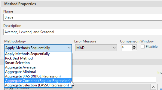
Aggregate Combine (Regular Regression)
Regression of the time series against the forecast from the different methods.
'Combine' means the regression of all the selected methods. Based on the forecasted value, Aggregate Combine runs a simple regression against historical actuals.
This uses a regression method to aggregate the output from the methods. This aggregation method would fail if there are more methods than periods, otherwise it would use the historical fitted value against the actual to create a regression model. The future estimates from the method are used to create future forecast for the aggregates.
For example, if you have a good data, but your accuracy is struggling at 60%, you want to consider using this.
🚧 Aggregate Combine should not be used for sporadic because they have gaps and might behave like an average.
Comparison Window
The comparison window section has the forecasting windows options for selecting a percentage of periods to withhold from the engine when forecasting, and also the Flexible checkbox.

Flexible checkbox
Checking the Flexible checkbox will change the Comparison Window to a Dynamic Window.
This will adjust the Comparison window based on the size of the historical periods. The size of the window selected would be compared against the size of the historical period and if it would be reduced. The Comparison window size cannot be more 10% of the historical size and no less than 2. For example, is forecast data has 24 period and you select a window of size 10, that would be reduce to 2. 10% of 24 is 2.4 rounds down to 2, max(2,2)=2.
Forecasting Windows
When we forecast, we look at periods of history to try to predict what future periods will look like. Periods can be months, weeks, days, quarters, etc. We want to forecast this period.
Arkieva Statistical Forecasting helps forecasters by selecting a best method for predicting future periods. However, before Arkieva can do this we must specify a few things.
First, we select which and how many methods we want Arkieva to consider when we run the forecast.\ Next, we select the methodology. The methodology will select the best method.
Then, we select an Error Measure. The error measure is like a second methodology that uses a formula to generate the forecast.
Lastly, we select a percentage for the comparison window. This will help the system determine the size or number of periods to withhold from the engine when we generate the forecast. By us knowing what the withheld history data is, we will be able to determine how well the system performed in predicting the future period data.
📘
Selecting many methods and/or choosing a high number of windows can put strain on the system when generating the forecast. We recommend that you do not go over 10% when selecting windows. For example, in a weekly database there is three years of history; 52 times 3 is 156, 10% of which is 15.6. For that example, the window should be no more than 16.
To explain how Arkieva selects a best method from these many inputs when generating a forecast, we will use the following Excel example. For this exercise we have 36 periods of history, and 24 periods out into the future. Orange is the History, and Blue is Future.

We will create a method called Arima with Seasonality. We will then select MAD (Mean Absolute Deviation) as our error method and set our window to six percent. This will advance 6 periods of history into the future. By withholding periods 31 through 36 from the system, when we run the engine for the first time, the system will generate the forecast using the first 30 periods and forecast the last six periods.
To show how Arkieva will calculate the MAD, we will first manually calculate the MAD error on periods 31, 32, 33, 34, 35, and 36. And doing this, we will get six error measures. Then we will repeat this process, but instead of advancing the last six periods, we will advance the last five. Meaning, using MAD, the system will generate the forecast for periods 1 through 31, and advance periods 32 through 36 into the future.
We can now calculate the errors in these five periods (32, 33, 34, 35, and 36) based on what has happened historically, resulting in five brand new error measures.
We can repeat this process by advancing the last four periods into the future, then the last three, the last two, and then just the last period. When finished we will have 21 different error measures.
📘
This was all done using one method. However, to get the maximum effect from forecasting with Arkieva, you will most likely use multiple methods that you are interested in evaluating. Say you selected ten methods to be calculated with MAD for a window of six; Arkieva will use the above steps for the first method, then repeat it for the second method, then third, fourth, fifth, and so on. Each method will have 21 different error measures; however, the system will aggregate these numbers and give you one final forecast score. And by viewing these scores, you can determine which is the best method for forecasting by looking at the forecast with the lowest score. And once we have that selected method, we can use that method to forecast against the entire 36 period history.
Now with the following examples taken from Arkieva, we will show how Arkieva generates a forecast while using windows.
Using the below time series as an example, we can see it has a specific shape; it is sloping down but has some peaks. Keep in mind that the dark gray area is history, and the red line denotes the end of history. The white area is for future periods.
For reference, Time Series 4 has no advanced periods out into the future.

For Time Series 5 Now we have copied Time Series 4 periods however we have advanced the time series forward four periods.

📘
By sliding the time series over, we have created leading zeroes. Leading zeroes are ignored by Arkieva and will not affect the outcome of the forecast.
Also, in this example there is a half month at the end of the time series, we will ignore this for the purpose of our exercise.
Now we will generate the forecast using the method we defined, Arima with Seasonality, MAD error measure, and four windows. Now we will select Time Series 5, and go to the Data tab.

Since we already know the history of these four periods, we can focus our attention on only these four periods. We will export this time series to Excel. Then, we will calculate the MAD for these four periods to get four absolute errors.


The error in the first period is 95. The error in the second period is 275, third is 369, and fourth is 261.
We can now repeat this process for the remaining Time Series. Remember, for Time Series 5 we have advanced time series forward 4 periods, and here in Time Series 6 we have advanced the time series by 3 periods. We will again go to the Data tab and export this time series to Excel and calculate the errors but only for the three periods we have advanced into the future forecast. We now have three absolute errors.

📘
Notice that earlier when we were discussing how in Arkieva we can set windows to trick the system into thinking specific historical time periods were out in the future, that the pattern was sloping down to the right. However, when we manually slide historical time periods out into the future, the pattern slopes down to the left.
Next, we will go to Time Series 7. Here we have advanced two periods forward into the future.

And we will perform the same error calculation to now get two absolute errors.

And lastly, we will go to Time Series 8 where we have advanced one period into the future. And we will get one absolute error.


So now we will sum these error values and get a score of about 2056.70.


That is the first part of the process to show how Arkieva performs these calculations in the background, however there is a second part to this process that we can also perform on our own using Excel.
If we go back to the forecast and hover our mouse over the Errors graph, we can see our Arima with Seasonality method returned an absolute error of 4985.74. However, when we calculated the SUM of our absolute errors, we got 2056.70.

The reason being Arkieva takes the cumulative sum of all the windows, or in other words each of our calculated absolute errors.


Cascade
In Arkieva statistical forecast the comparison window allows us to split the data into training data and validation data.
Cascading allows us to iterate through periods in the comparison window each time adjusting the training periods and the validation periods. The error is calculated as an aggregate of each of the error form each iteration.
Cascading was always enabled by default, however now you can disable cascading by unchecking the enabled checkbox under the Cascade option.
For example, if one has 36 periods of data and a window size of 4 periods then we have the following iterations:
- Window period 1: training period would have 32 periods and validation period would have 4 periods.
- Window period 2: training period would have 33 periods and validation period would have 3 periods.
- Window period 1: training period would have 34 periods and validation period would have 2 periods.
- Window period 1: training period would have 35 periods and validation period would have 1 period.
- The validation error from each iteration is used in the calculation of the error measure that determines which method is selected as the best method.
- Final period: training period would have 36 periods, in this run there is no validation.
When cascading is off, there is no iterations within the window periods needed and as a result only 2 runs are required. The error measure is calculated using 32 periods for training and 4 periods validation.

Running the forecast with cascading disabled will offer the same or close to the same forecast accuracy as running the forecast with cascading enabled.
Disabling cascade will also return the forecast results faster than when cascade is enabled because it is not performing as many calculations.

In the example below you can see that when Cascading is set to ON is it very similar to when Cascading is set to OFF. Also notice the runtime has been considerably reduced by turning Cascading OFF.
| Product | Cascading | Methodology | Run Time | Forecast Error Score | Error Measure |
|---|---|---|---|---|---|
| Time series data with 85,849 tuples | ON | SMART | 26min 19sec | 47.2% | HWGHTD |
| OFF | SMART | 7min 50sec | 47.5% | HWGHTD |
In the next example below you can see that when Cascading is set to OFF, even though the error score has increased by 7%, the runtime is still considerably reduced by 2 hours.
| Product | Cascading | Methodology | Run Time | Forecast Error Score | Error Measure |
|---|---|---|---|---|---|
| Time series data with 85,849 tuples | ON | Pick Best | 3hr 56min | 25.6% | HWGHTD |
| OFF | Pick Best | 1hr 24min | 32.2% | HWGHTD |
🚧 Pros and Cons of disabling cascading.
Enabling cascading will offer some level of consistency in terms of Arkieva selecting the best method for your forecast. As the system goes through iteration of the comparison window combinations, the system may select a different best method. And the best method that appears more consistently and has less errors will be the one selected to forecast against.
A forecast run without cascading will not be as thorough, however if you know your data is accurate, then your forecast will be run much faster and with similar accuracy. Data that is considered 'good' would be data with a consistent trend from period to period. However if your data is intermittent, disabling cascading is not recommended.
Fox Seasonal
Seasonal using sin/cos\ We call this method “FS” – fox seasonal. It is used in two places:
- To declare if a time series of demand history is or is not seasonal (not in smart forecasting, but other modules)
- As one of the forecasting methods to be selected as “best”
It is a method that optimizes. It uses the least squares optimization method; mulreg routine in the Arkieva library.
- The dependent (Y) variable is demand history.
- The only true independent (X) variable is an integer for each period or time bucket called “k”. If we have 36 months of data starting in January, k is 1 to 36, inclusive. If we start in March, then k is 3 to 38, inclusive.\ The k can be converted to a common unique integer for each month called kc, where kc=mod(k,12), where 12 is the number of months in a year. In the case where start with march, kc is (3 to 12),(1 to 12),(1 to 12),(1 to 2)
- It has 4 synthetic variables: Sin(4w), Sin(2w), Cos(4w), Cos(2w); where w is π×k/cyc or π×kc/cyc
The full linear estimate equation is:
Y ={b0} + {b1×k} + {(b2×sin(4w) + (b3×sin(2w) +(b4×cos(4w) +(b5×cos(2w)}
Y = P1 + P2 + P3
The purpose of P3 is to capture any seasonality with linear combinations of the 4 synthetic variables (using sine and cosine). See figure below.
- If just P1 is a good fit, then the average of y is a good fit
- If just P1 and P2 are a good fit, then a linear trend is a good fit
- If the first two options do not produce a good fit, but the addition of P3 generates an improved fit, then we conclude there is seasonality; P3 is needed to go with P1 or (P1 and P2).
📘 Note
To be declared seasonal, it needs to be substantially better fit then linear trend, but it still may not be a good fit.
- For forecast, its selection as best will depend on the method used to pick best. A fit example from some randomly generated is posted below.
History
There are a number of papers in health care pointing to this method as an easier alternative to other methods to assess seasonality:
Studying seasonality by using sine and cosine functions in regression analysis


Causal Forecasting
Error Measures
Related Articles
Multiple Regression
Multiple regression is a statistical forecasting technique that uses multiple independent variables to predict the value of a dependent variable. Multiple regression allows for multiple predictor variables. Any prediction of the dependent variable ...Forecast Performance
The following is a list of Performance Metrics. Bias Total bias shows how many units your forecast is deviating from the actual sales values in absolute terms and whether the forecast is biased towards overestimating or underestimating the actual. ...Forecast Methods
Introduction To create a custom method to be used in the Statistical Forecast component, click the New button located in the Forecasting Methods ribbon. The new method with the name 'New Method' will appear under the Custom Methods category. Under ...