Multiple regression is a statistical forecasting technique that uses multiple independent variables to predict the value of a dependent variable. Multiple regression allows for multiple predictor variables.

• Any prediction of the dependent variable includes all the independent variables, even if they are statistically insignificant. This if for example applies all five independent variables are used to estimate a regression model. To estimate slope coefficients, correlations between these variables are considered.
• The intercept term must also be included in any prediction of the dependent variable.

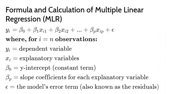
Formula for multiple regression:

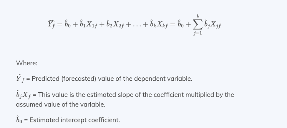
Each component means:

• Predicted Value: The value trying to be predicted using the regression model.
• Intercept: The predicted value when all predictor variables are zero; serves as the baseline level of the dependent variable.
• Slope Coefficients: Estimated values indicating the expected change in the dependent variable for a one-unit change in each corresponding predictor variable, with other variables held constant.
• Predictor Variables: The independent variables used to predict the dependent variable.
• Sum of Products: The total predicted effect of the predictor variables on the dependent variable, calculated by summing the products of each slope coefficient and its corresponding predictor variable value.

Various forecasting methods similar to multiple regression.

External Indicators

In multiple regression, external indicators are variables that are not part of the primary dataset but are included in the regression model to improve its accuracy and predictive power. By incorporating external indicators, the model can account for factors outside the primary dataset that affect the dependent variable, leading to more accurate predictions.

Examples:

• Economic Indicators: GDP, inflation rates, unemployment rates.
• Demographic Data: Population size, age distribution, income levels.
• Environmental Factors: Weather conditions, pollution levels.
• Market Trends: Stock market indices, commodity prices.
• Policy and Regulation: Tax rates, regulatory changes, political stability.

Implementation of multiple regression using external indicators

Arkieva provides the flexibility to add external indicators and apply different forecasting methods using external indicators.

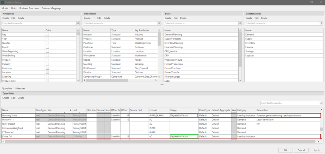
To fully utilize the potential of external indicators, they must be updated in Arkieva through the Setup Manager. The external indicator should be added as a quantity, loaded into a star, and the field "Usage" should be updated to "RegressionFactor". Multiple quantities at a time can be marked as Regression factor. This step is necessary so that they can be later used in multiple regression forecast methods as an external factor.

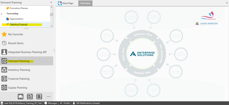
Within the Demand Planning section in Navigation, Open Statistical forecast component within the Forecasting category.

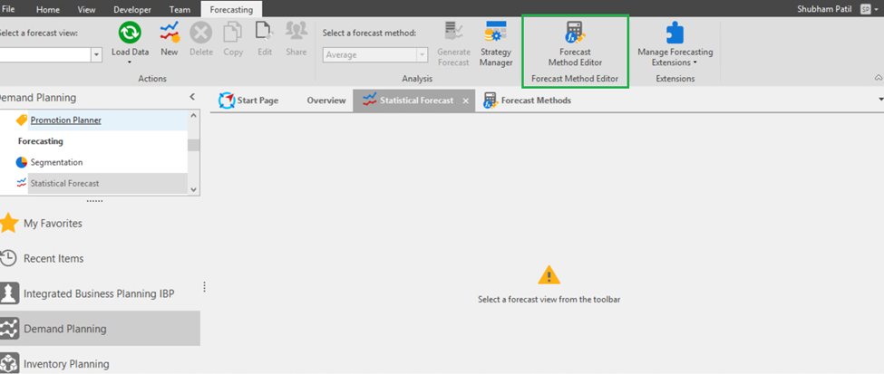
Click and Open the Forecast Method Editor.

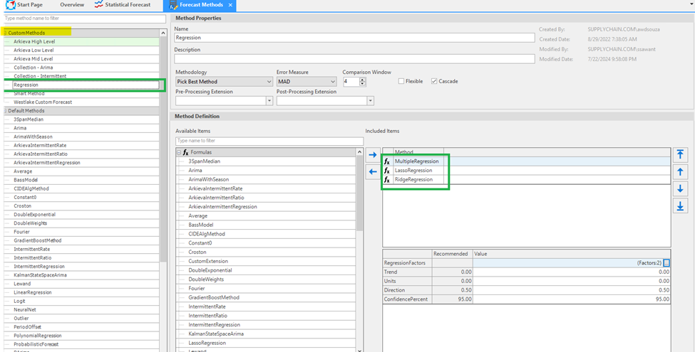
Arkieva provides an option to build customized forecasting methods within the Forecast Method Editor by clicking the “New” icon. A new custom method can also be created from a copy of existing custom method using the “Copy” button and saving the changes. We have already created a custom method “Regression” by adding Multiple, Lasso and Ridge regression.

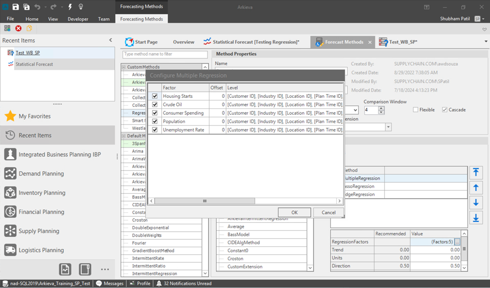
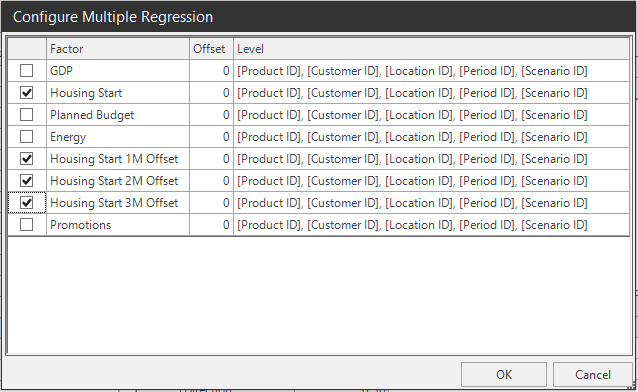
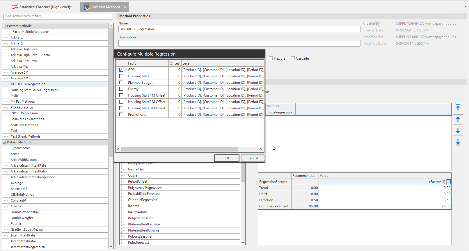
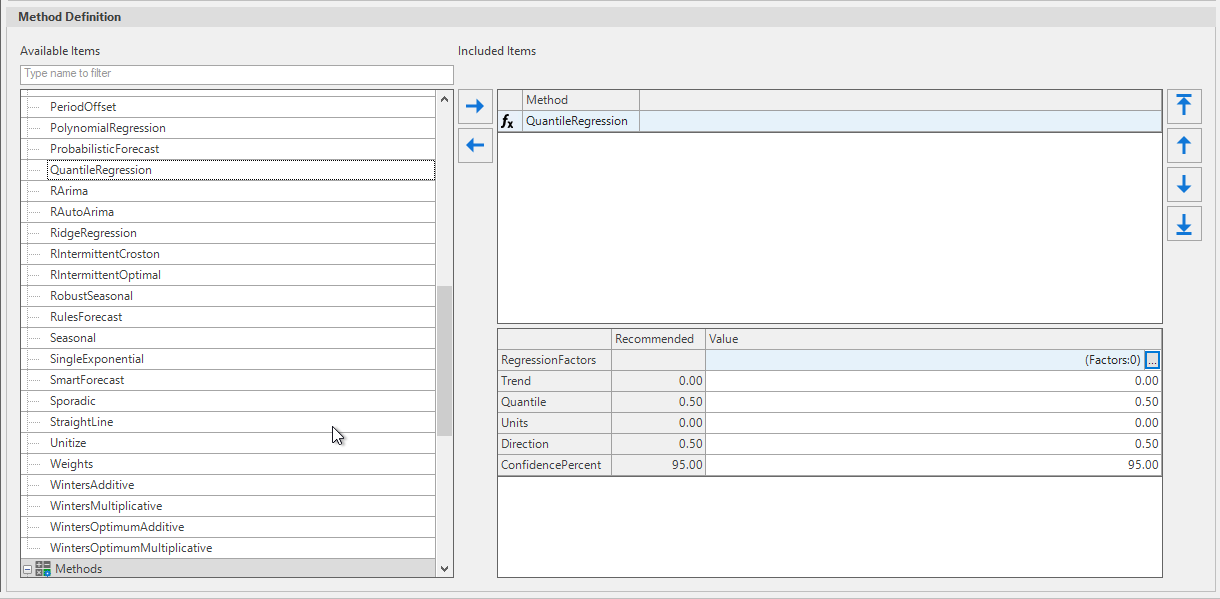
Clicking on Multiple regression method, there are parameters that can be modified to generate the Results Regression Model:

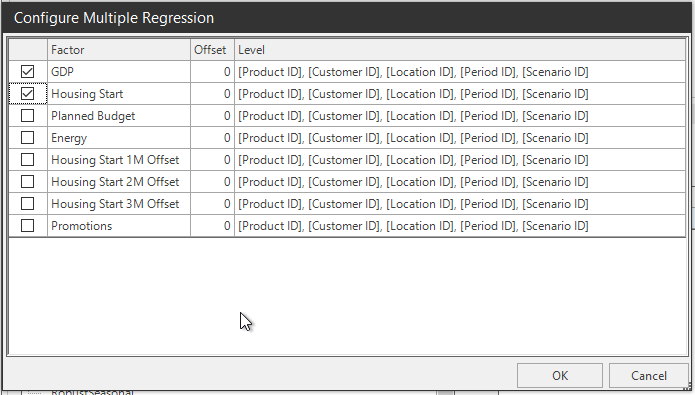
Factor: The quantity/quantities added in setup manager will be visible in the list of factors in the “Configure Multiple Regression” popup window. Check the checkboxes to select as many external indicators as required.

Offset: The effect of the regression factor on the forecasted quantity can be adjusted using the Offset factor available in the pop-up window. This adjustment makes the regression factor a leading indicator. The offset value is crucial because in most cases the influence of a causal factor on the forecasted value is not instantaneous.

Level: An external indicator may not impact the lowest level of data, i.e., the Tuple, but it could affect other data levels. The data level selection for the specific external indicator can be adjusted here.

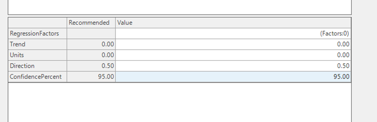
Trend:

• Units and Direction: For example, if the forecast needs to be generated in whole units for Truckload quantity, modify the parameter “Units” to round the forecast to the desired number of units. Additionally, the “Direction” parameter allows for whether the forecast should be rounded up, rounded down, or set to zero.
• ConfidencePercent: This is a parameter measure that can be updated to desired level. It indicates the percentage certainty that the true value of the forecasted variable falls within the specified confidence interval.

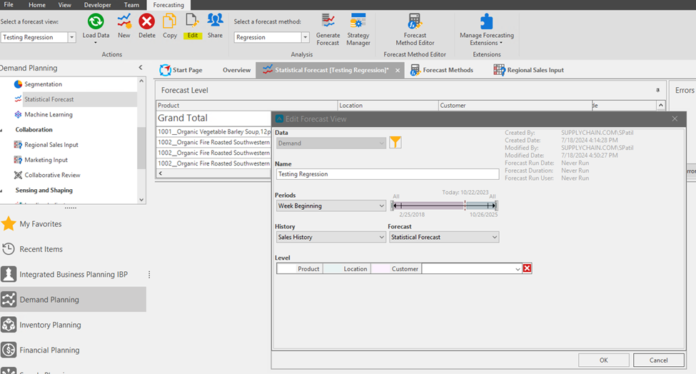
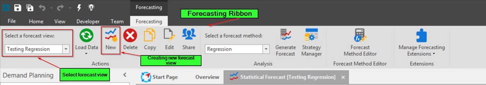
Next, select a forecast view and forecast method (Regression – which is a custom forecasting method with multiple regression) in the Forecasting ribbon.

Click on Edit View and update the Data, Name, Periods, History(quantity), Forecast(quantity) and Level as required.

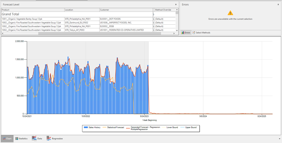
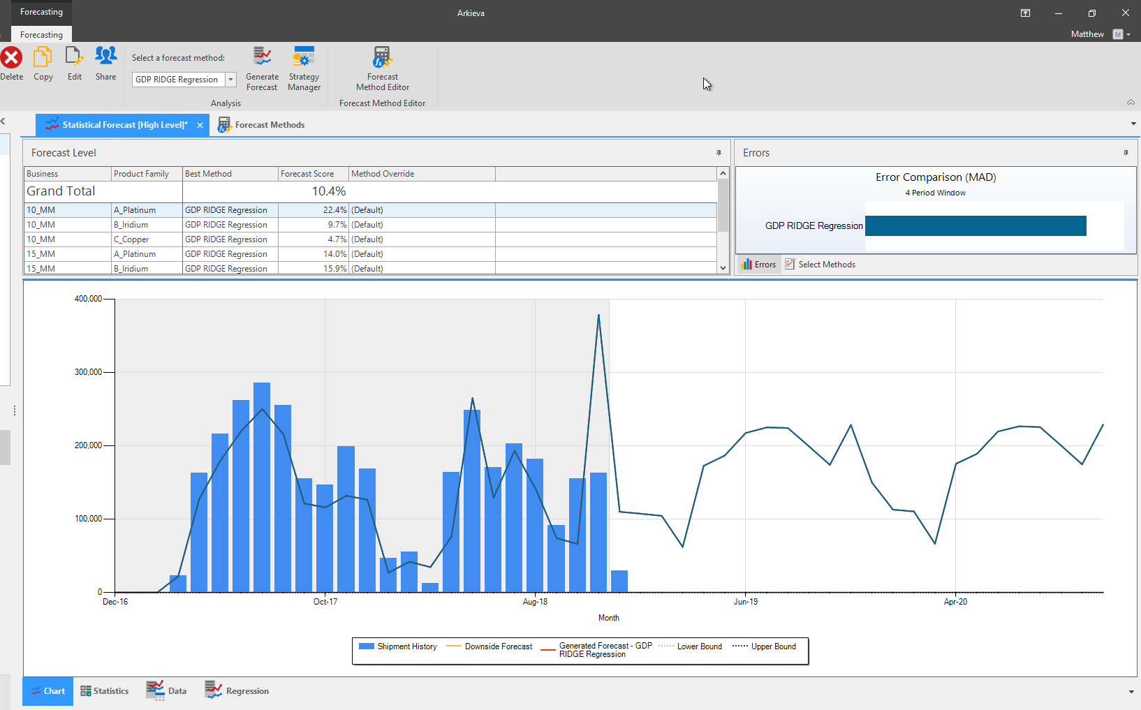
Click on Generate forecast and observe the result.

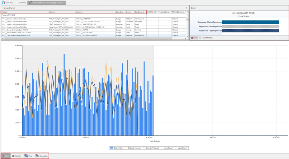
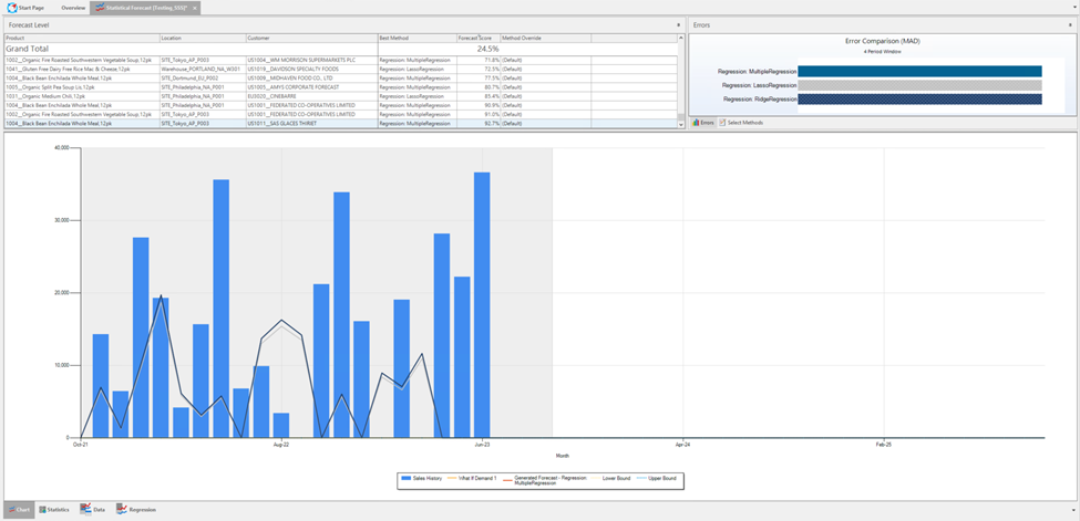
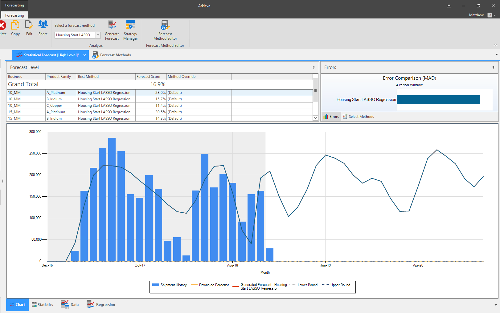
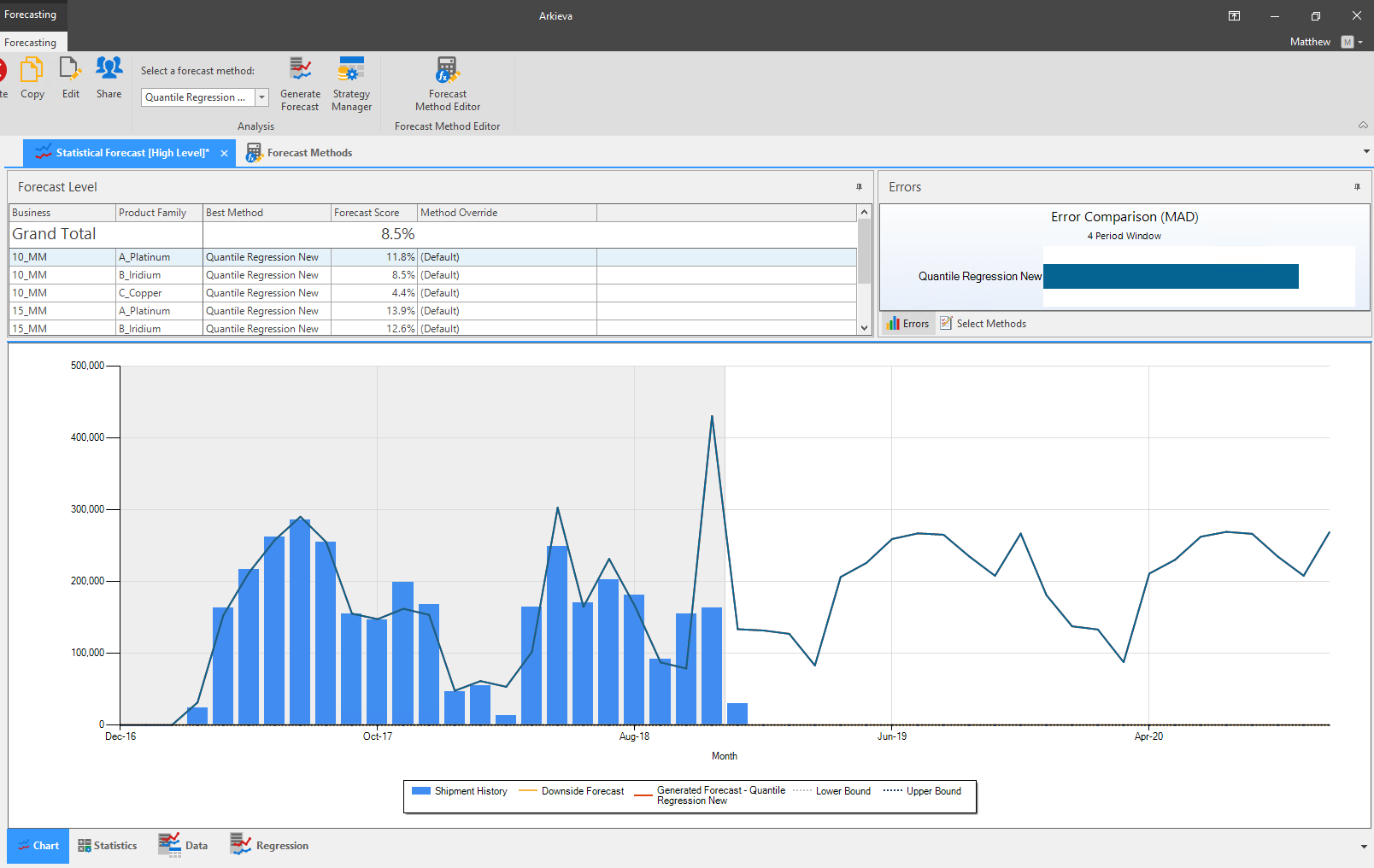
The Chart tab displays the results of the generated forecast in graphical form.

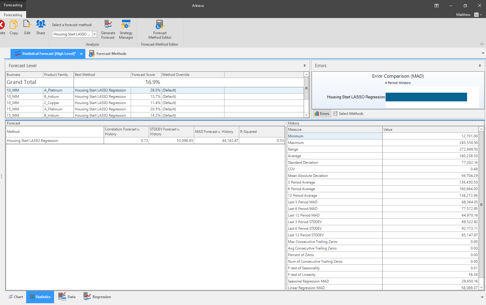
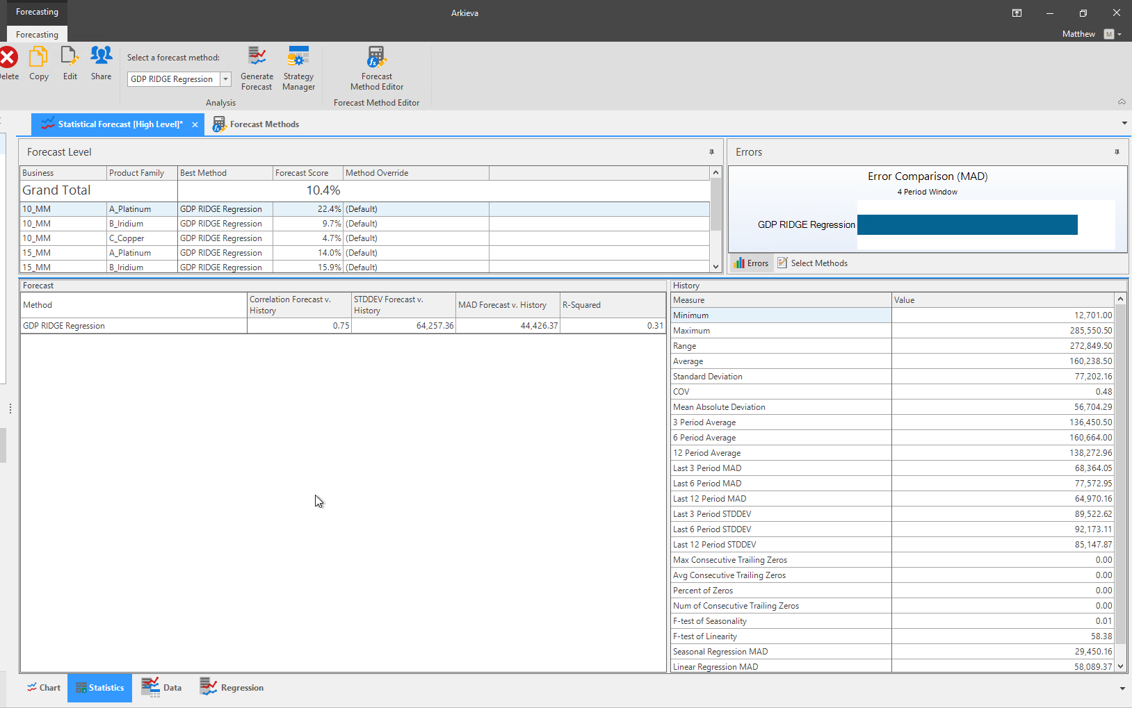
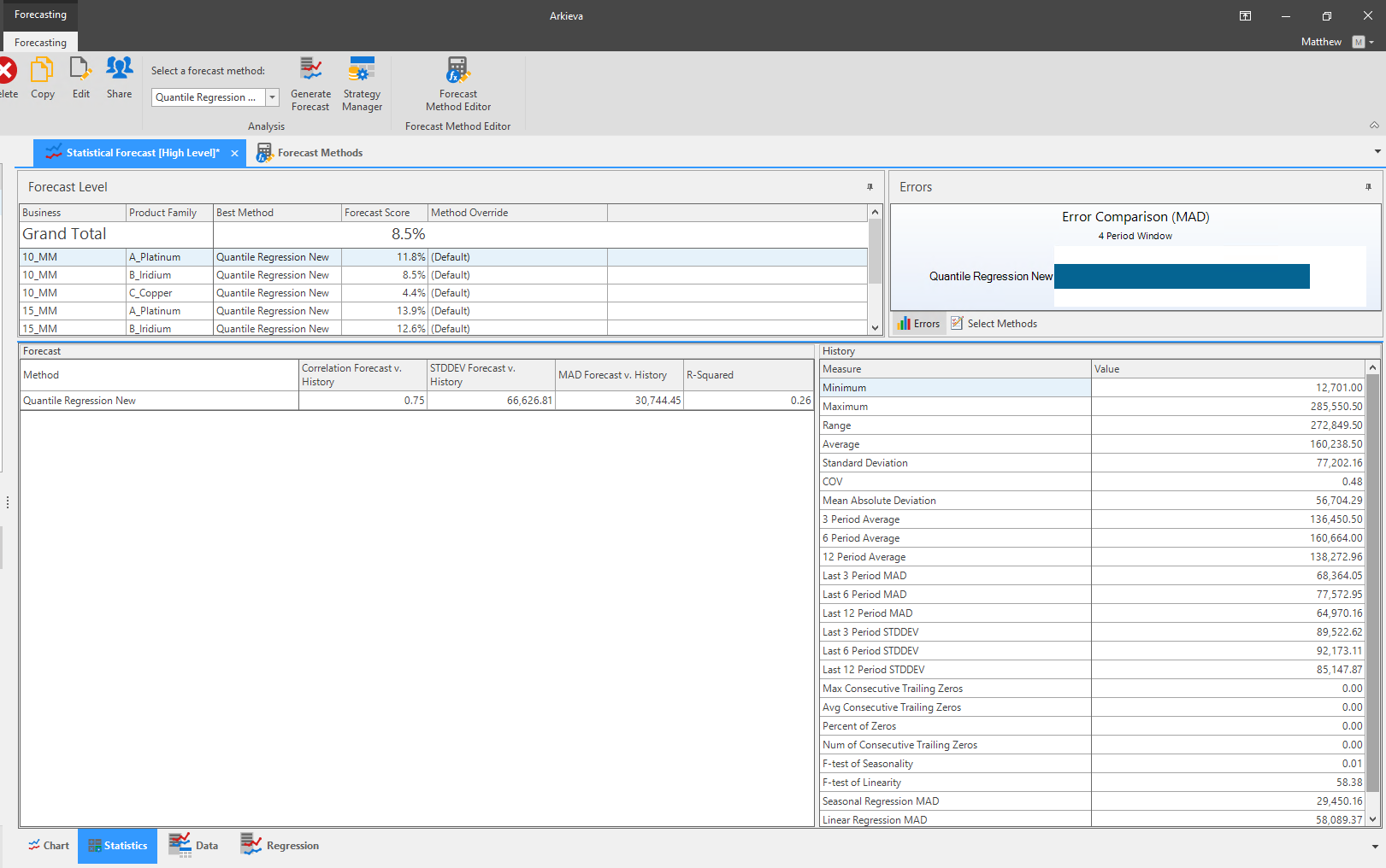
The statistics tab displays the statistical calculations generated while calculating the forecast.

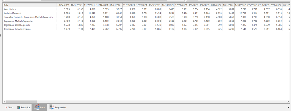
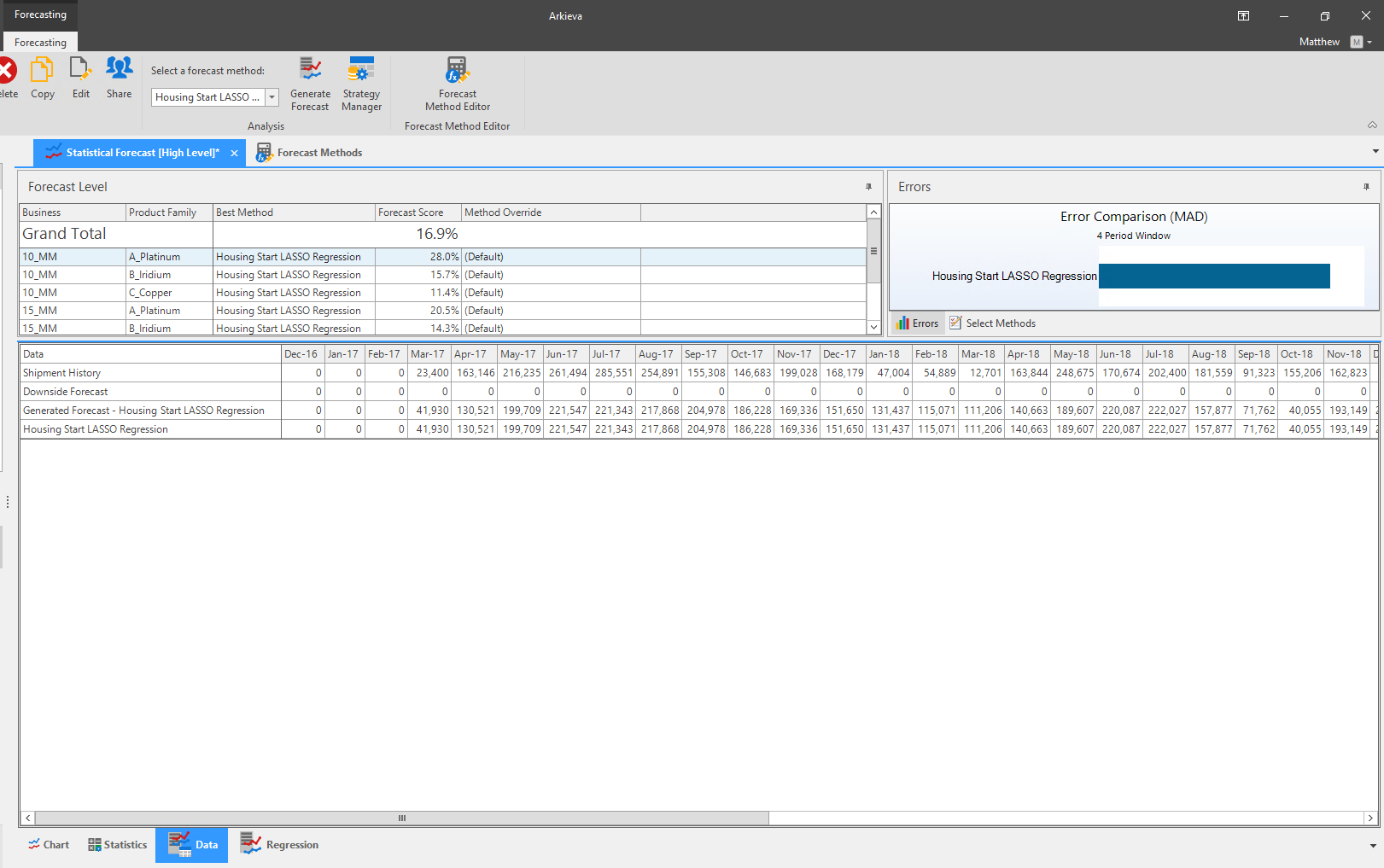
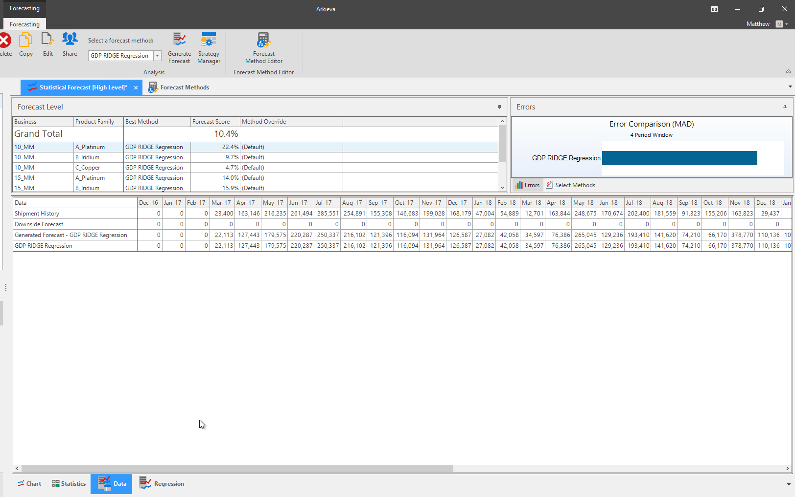
The Data tab displays the actuals data with forecasted quantities using all the methods presented in the custom method.

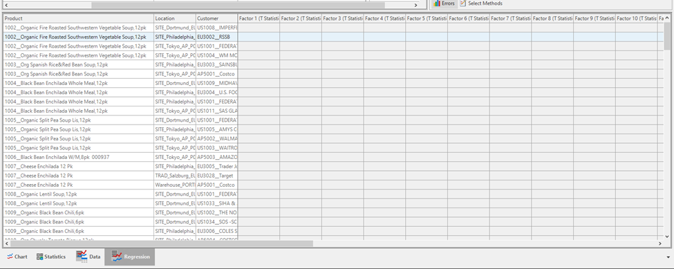
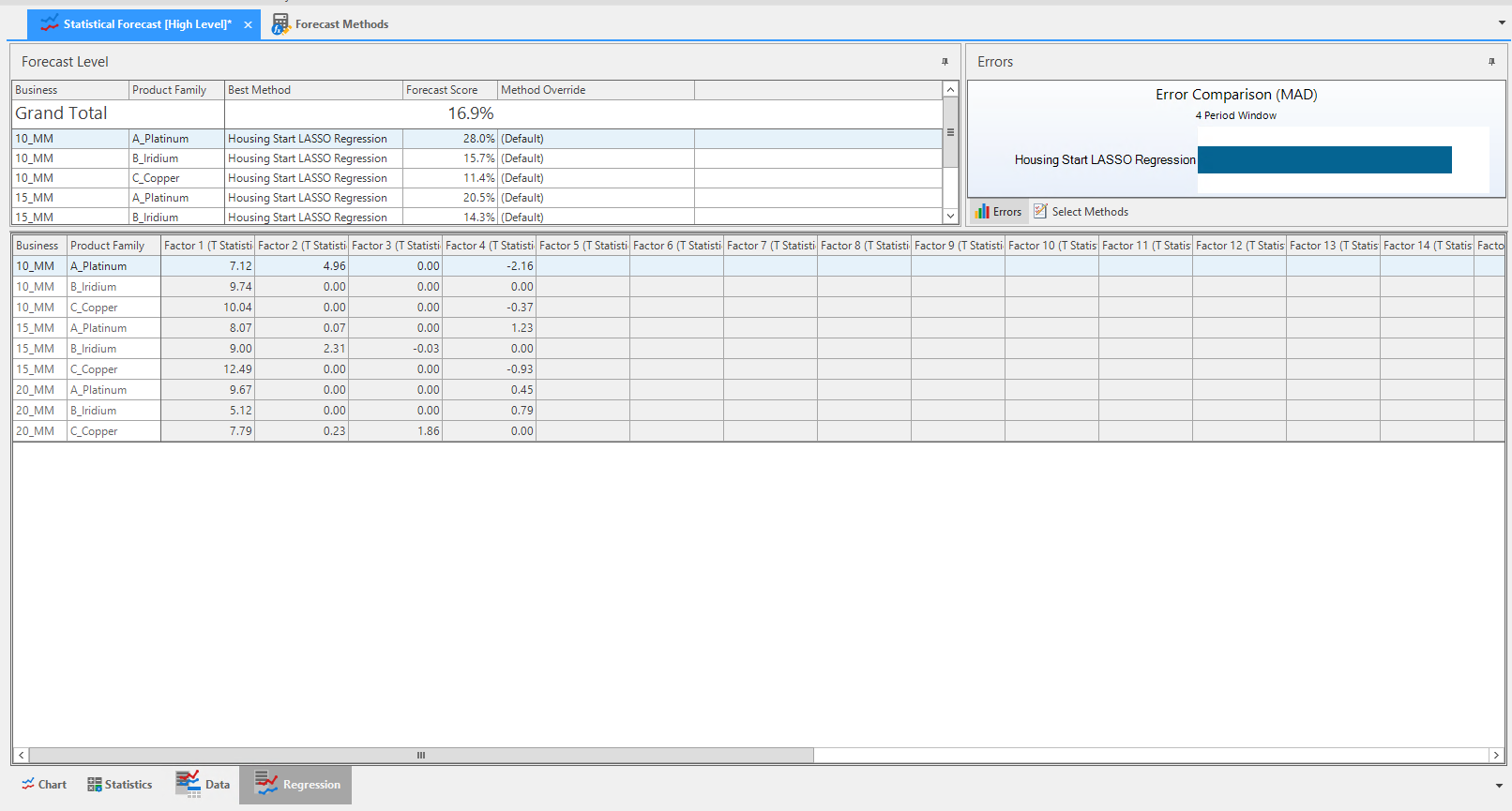
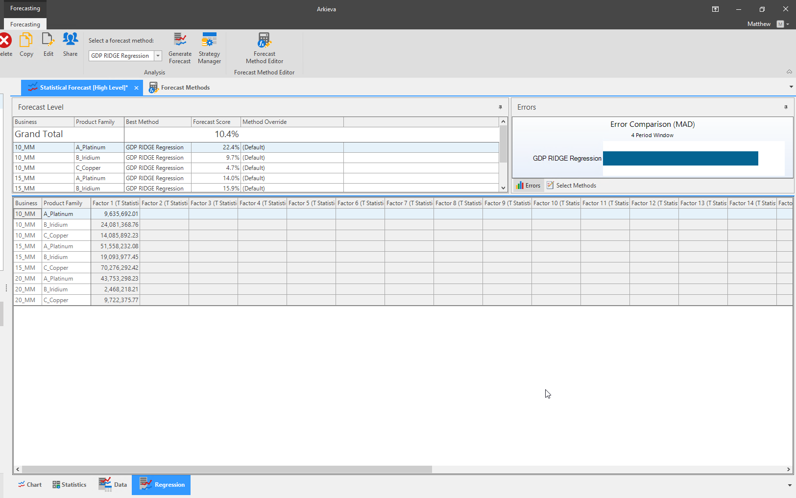
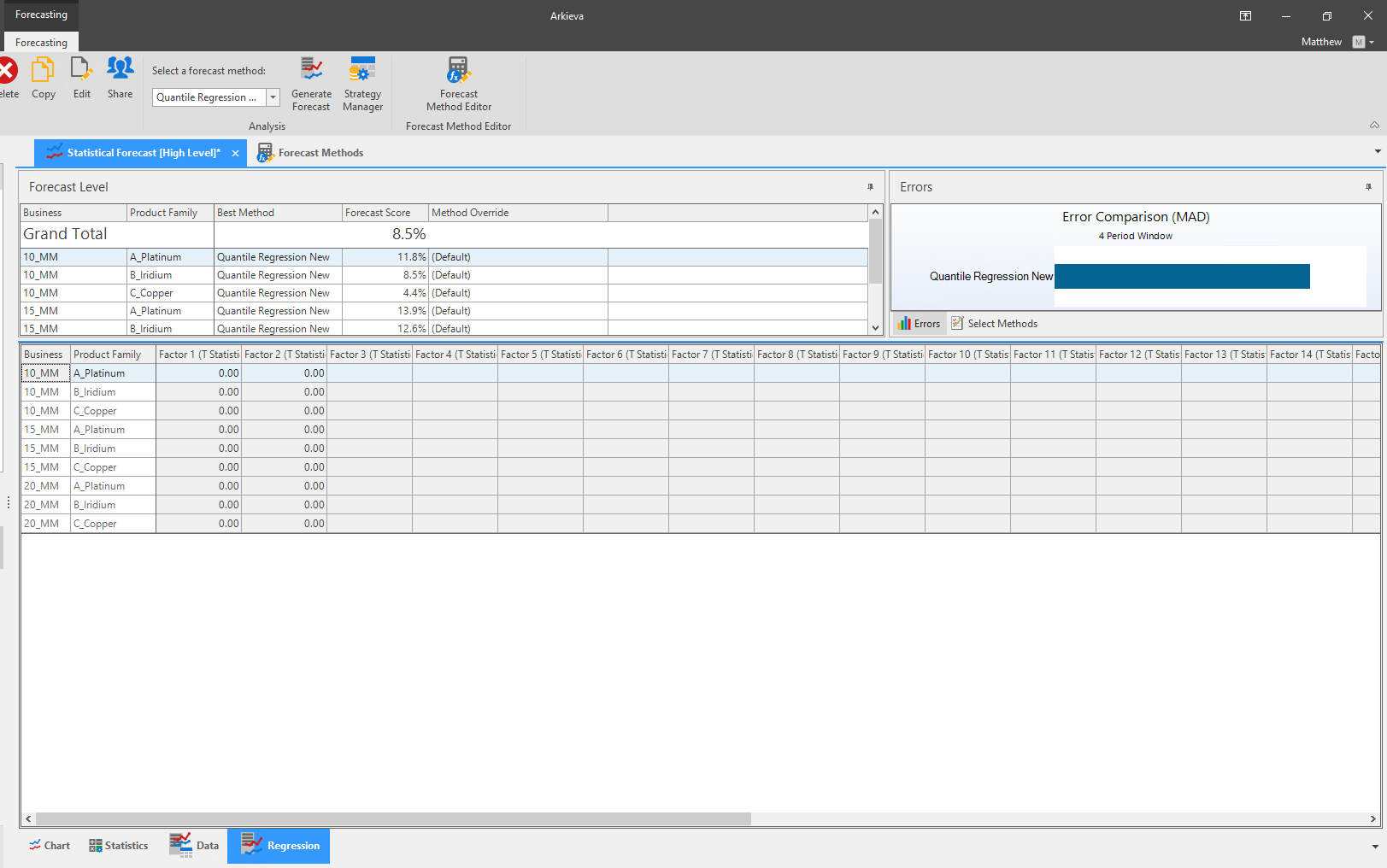
The Regression tab displays the regression statistics, t-value factor at level selected in the Edit forecast view.

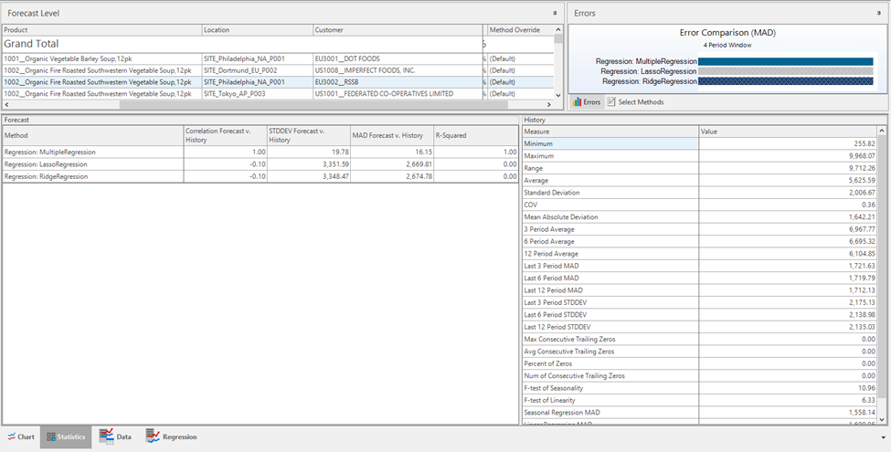
After observing the error comparison window, if not satisfied with the generated forecast, there is the option to compare different forecasting methods. By creating multiple subsets of data in a new view, the user can apply and evaluate various forecasting methods to select the most suitable one.

Multiple Regression in forecasting

Multiple Regression is a statistical technique analyzing the relationship between one dependent variable and several independent variables (predictors) and is used to find a linear relationship between variables in situations with multiple independent variables.

Multiple Regression forecasting methods can be used when the reason for peaks in historical data are already known, and those peaks are quite significant compared to the base sales. The regression model can then help to generate forecasts where the peak position occurring in the future can be identified, while continuing the baseline for the rest of the periods. Hence it is useful for any certain event in future like in the past i.e. Christmas, promotion, special days etc.

Requirements\ Constant factor (for baseline sales):

• Assign 1 for all past periods where there is any sales > 0.
• And Fill up all the future periods with 1. ( in case you want to have a constant base sales for all future periods)
• Dummy Variable: You would need to specify or pin point those events in the past by using a dummy variable like 1,0,1,0
• And Point periods in the future where you would expect them to repeat.
• Create a quantity for it and publish the dummy variables using a function that can identify peaks. (i.e. insert 1 if the sales is 10 x of base sales else 0)
• Provide source table and column and Date like usual quantities and assign that quantity as factor under usage in SETUP Manager.
• Select Forecast and Regression and click Apply.

Formula

Understanding dependent and independent variables

• Dependent Variable: The variable being forecasted (Demand).
• Independent Variables (Predictors): External factors influencing the dependent variable. Examples: Marketing spend, economic indicators, seasonal factors, housing starts, crude oil prices.

Application in Forecasting

• Predicts future values of the dependent variable based on multiple independent variables.
• Helps understand how various external indicators influence the forecast.
• Useful for complex forecasting scenarios where multiple factors affect the outcome.

Advantages of Multiple Regression in Forecasting

Considers multiple influencing factors simultaneously and provides a more comprehensive view of potential future outcomes. Can also improve forecast accuracy by incorporating relevant external variables and allows for quantification of each predictor's impact on the forecast and helps in identifying the most significant factors affecting the forecast.

• Example: Demand Forecasting.
• Dependent variable: Future Demand.
• Independent variable: Economic indicators (GDP, Inflation rate, unemployment rate), Seasonal factors.
• Multiple regression will help us predict how external factors may affect demand and will help us in right sizing inventory and strategic planning.

Statistical Forecasting

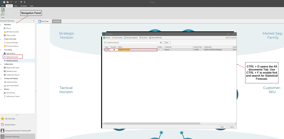
Statistical forecasting module can be launched by clicking on Statistical forecasting in Navigation Panel or can be access by Using CTRL + D (Browse all documents).

After launching Statistical forecast, create a new forecast view which will be available in the forecast dropdown or select a forecast view from the forecast dropdown. In this example there is already a created view named "Testing Regression".

Once the forecast view launches, the forecast level in the forecast section can be viewed. The Errors tab will display errors for various methods used for forecasting. At the bottom of the window are the options for Chart, Statistics, Data and Regression.

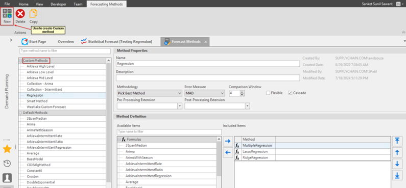
Before we dive into statistics and data, let's look at the forecasting method we selected. Currently, the forecast method is set to regression; to look at how regression is setup and to make changes, click on the Forecast Method Editor button in the forecasting ribbon.

The forecast method editor exposes all the default methods available in Arkieva. There are also custom methods available. Custom methods can be created by clicking on New and setting the Method properties and definitions. We have created a Custom Method called Regression. The methodology is set to best pick methodology and Error measure is MAD. We add Multiple, Lasso and Ridge regression as methods.

To configure the Regression method, Select the regression method and click on the ellipses button in front of regression factor.

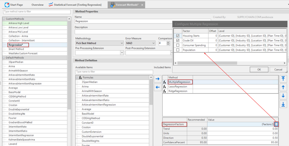
Regression factors like Housing Starts and Consumer Spending are external factors to consider while forecasting demand. For the External factors to be listed in the “Configure multiple regression” tab, we must add these external factors using Setup Manager under teams. In setup manager, click on model and add these external factors as quantities, Select the appropriate Data type, Start, Unit, etc. and enter usage as ‘RegressionFactor’.

Once the external factors have been added, configure regression factors and click save. Go to statistical forecast, Select the appropriate view and forecast method and generate forecast.

LASSO Regression

LASSO (Lasso) is an acronym for Least Absolute Shrinkage and Selection Operator. Lasso is a regression method that performs variable selection to improve accuracy. Lasso only includes the variables likely to improve the accuracy of the Regression model. Similar to Regular Multiple Regression, Lasso has the same inputs and the same outputs, the only difference being the variable selection. It is a regression technique that imposes constraints on the coefficients. It is employed for causal forecasting and acts as a variable selection tool, minimizing the impact of unstable variables while having the capacity to eliminate many variables.

• Regression of the time series against the forecast from the different method.
• Select the best method output to be included in Regression.
• Reduces the influence of unstable output from a method.

Lasso selects factors that have a strong correlation with the independent variable. It does so by kicking out methods and uses optimization (co-ordinate descent) which looks at one variable and tries to converge.

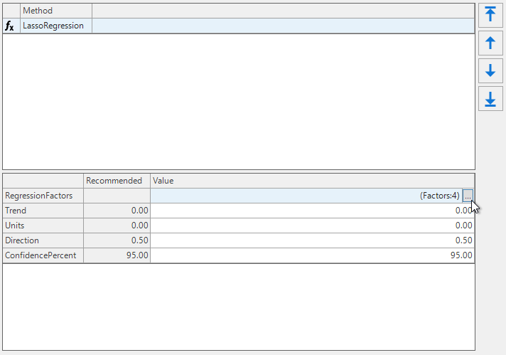
Going back to the Statistical Forecast tab, select the created Lasso regression forecast method and generate the forecast. Below are the different ways Lasso regression can be seen and how it effects the forecast in the Chart, Statistics, Data, and Regression tabs.

📘 Lasso and Ridge

Both Lasso and Ridge have a parameter called "Shrinkage" which helps control how it eliminates things. Use this method if you are struggling with which methods to eliminate.

Ridge Regression

A regression approach where coefficients are constrained. It is used for causal forecasting, reducing the impact of unstable variables and effectively managing unstable data.

• Regression of the time series against the forecast from a different method.
• Reduces the influence of unstable output from a method.

Ridge Regression introduces bias into a regression. By adding a degree of bias to the regression estimates, Ridge regression reduces the standard errors. The intent being the net effect will give estimates that are more reliable. This is like the regular Multiple regression with a bias, has the same inputs and the same outputs, the only difference is the variable selection.

Going back to the Statistical Forecast tab, select the created Ridge regression forecast method and generate the forecast. Below are the different ways Ridge regression can be seen and how it effects the forecast in the Chart, Statistics, Data, and Regression tabs.

📘 LASSO and RIDGE

The above generated forecast needs lots of work and fine tuning.

Apart from multiple regression, we have numerous regression methods in Arkieva. But for now, we are considering Ridge and Lasso regression. Lasso and Ridge regression are used when we have many factors that influence our forecast, and we want to make our forecast more accurate. For example, consider each factor as a voice in a noisy room. Regular regression tends to listen to all voices equally whereas Lasso and Ridge act as selective hearing aids and help us focus on voices that matter the most. But there are differences between Lasso and Ridge.

Lasso is very strict with the selection criteria i.e. it completely neglects some of the least important factors, Lasso can be used when you want to only consider the most crucial external factors.

Whereas Ridge regression is gentler with its selection criteria I.e. it won’t remove the factors entirely but will reduce the influence of such factors on our forecast. Ridge can be used when we want to consider all the factors and adjust their influence on our forecast.

While predicting sales for Ice cream, Lasso might completely ignore factors like day of the week whereas Ridge will consider day of the week and will give more importance to temperature.

Quantile Regression

A Quantile is a proportion of data that is less than the quantile values. For example, 0.4 quantile of a sample of weights would mean 40% of the weights are lower than the sample of weight, and 60% are higher than the sample of weight.

Quantile Regression is a type of regression analysis used in statistics and econometrics. Whereas Multiple regression estimates the conditional mean of the response variable across values of the predictor variables, quantile regression estimates the conditional median (or other quantiles) of the response variable as a function of the regression factors. Quantile regression is an extension of linear regression used when the conditions of linear regression are not met.

Quantile regression is considered more robust than multiple regression and can be used in place of Multiple regression.

Quantile regression as implemented in Arkieva has the same parameters as multiple regression except for the Quantile Parameter. The Quantile parameter takes values greater than 0 and less than 1. The 0.5 quantile is the median. The default quantile is 0.5.