Outliers
Understanding Outliers
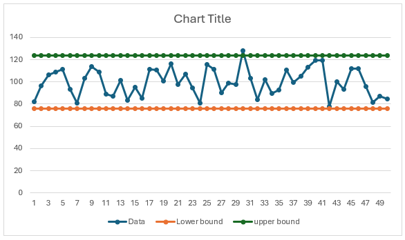
An outlier is a data point that differs from all data points, that data point is considered an anomaly. To find an outlier, we define boundaries and any data point outside of this defined boundary is considered an outlier. The boundary is defined in the form of a lower and upper boundary. Any data point greater than the upper boundary or lower than the lower boundary is considered an outlier.
The boundaries are defined based on confidence that any random data point would fall within the defined boundary. This confidence is expressed in the form of a probability, so it defines the probability of the data point falling within a range, sometimes it is defined as the probability that any random data point would fall outside the range.\ Given the probability, it is used to determine the values for the lower and upper boundaries.
Example 1: if we consider the height of people across the world and we consider 95% of the population to be of normal height. We can assume that an equal number of people would greater the upper boundary and same number of people would be lower than the lower boundary. A sample of heights of people shows that 2.5% of the population are less than 4 feet in height and another 2.5% are more than 7 feet in height. This means 95% of the sample are in the range of 4 feet and 7 feet. Anybody with a height out of the 4 feet to 7 feet range is considered an outlier, either too tall or too short.
There are several ways of determining if a data point is an outlier, but all the methods have in common a probability confidence is defined and that is used to determine the boundaries. Here are some general steps for detecting an outlier.
General Outlier detection steps:
- Cutoff error (expressed either as probability confidence or probability error)
- Central tendency measure (e.g. mean, median, mode etc.)
- Dispersion measure (e.g. standard deviation, range, Quantile range, interquartile range etc.)
- Find acceptable range, a function of the dispersion measure and central measure. The cutoff error is used to estimate these values.
- Lower bound
- Upper bound
- Data outside acceptable ranges are considered outliers.
- Accept or reject outliers’ correction recommendation.
Outliers in forecasting
A forecast data is called a time series, it is sequential, which means current activity may be dependent on past activity. Time series may have both seasonal and linear trends. For example, data may show that volume spikes every December and may be at its lowest in June. So, outliers in a time series can be defined as a data point that differs from expected trends in the data. For example, if in a period data expected to peak but it appears much lower than expected, this may be flagged as an outlier.
Due to the trends in a time series, normal outlier detection process may not consider the trends in the data and would likely to insensitive to outliers due the existence of trends. Normal outlier detection process would mistakenly flag or ignore a few data points as outliers when these are just reflections of the trends in the data or consider a data point normal when it is an outlier.
Outlier detection steps for time series:
- Cutoff error (expressed either as probability confidence or probability error)
- Remove all known trends in the time series data, so all that is left is a residual with no trends. Below are some steps for removing trends.
- Decomposition method. Time series data can be decomposed into Seasonal, trend and error portion.
- Use a forecast method that is insensitive to extremes of data and likely to capture the trends in the data.
- Use average as the forecasted information, this is equivalent to the traditional outlier detection data preparation.
- With the residual data, use the general steps for detecting if there are any outliers in the residual data.
Arkieva Outlier Implementation:
We split the implementation is 2 steps, the first step is data preparation (how errors are estimated) and the next step is the choice of method used to determine outliers.
We have 3 possible ways to prepare data (parameter SelectType):
- Use Robust Seasonal Forecast to generate the errors (SelectType = 1)
- Use raw data, like setting forecast to the average (SelectType = 2)
- Remove both Seasonal and other trends from the data aka Decomposition (SelectType = 3)
We have 4 methods for estimating outliers (parameter Run Option):
- Assume a normal distribution and use the classical method (RunOption = 2)
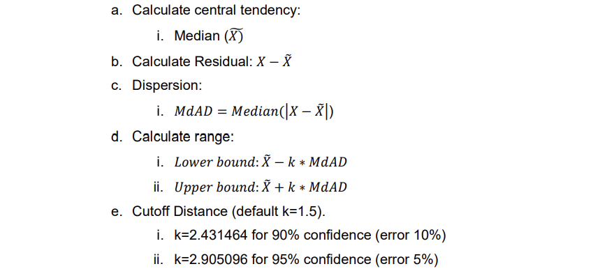
- Calculate central tendency:
- Mean (X)
- Dispersion:
- Standard deviation = Std (X)
- Calculate range:
- Lower bound: Mean (X) - k* Std
- Upper bound: Mean (X) + k* Std
- Cutoff Distance (default k=1.5)
- K=1.64 for 90% confidence (error 10%)
- K=1.96 for 95% confidence (error 5%)
-
Median Absolute Deviation (MdAD) method (RunOption = 1)
-
Calculate central tendency:
 2. Calculate Residual:
  3. Dispersion:
 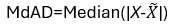 4. Calculate range:
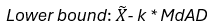
 5. Cutoff Distance (default k=1.5).
- K=2.431464 for 90% confidence (error 10%)
- K=2.905096 for 95% confidence (error 5%)
3. Sigma (or Mean Absolute Deviation, aka MAD) Method: (RunOption = 3) -
Calculate central tendency:
 2. Calculate Residual:
  3. Dispersion:
  4. Calculate range:
 5. Cutoff Distance (default k=1.5).
1. K=2.055435 for 90% confidence (error 10%)
2. K=2.456496 for 95% confidence (error 5%)
4. Inter Quantile Range (IQR) Method (RunOption = 0)
5. Cutoff Distance (default k=1.5).
1. K=2.055435 for 90% confidence (error 10%)
2. K=2.456496 for 95% confidence (error 5%)
4. Inter Quantile Range (IQR) Method (RunOption = 0) -
Calculate central tendency:
- Q1=First Quantile (X)
- Q3=Third Quantile (X)
-
 3. Dispersion:
1. IQR=Q3-Q1
4. Calculate range:
1. Lower bound:Q1-k*IQR
2. Upper bound:Q3+k*IQR
5. Cutoff Distance (default k=1.5)
1. k=0.712734 for 90% confidence (error 10%)
2. k=0.95295 for 95% confidence (error 5%)
3. Dispersion:
1. IQR=Q3-Q1
4. Calculate range:
1. Lower bound:Q1-k*IQR
2. Upper bound:Q3+k*IQR
5. Cutoff Distance (default k=1.5)
1. k=0.712734 for 90% confidence (error 10%)
2. k=0.95295 for 95% confidence (error 5%)
Parameter Combination:
In addition, there is a default value of SelectType = 0. This goes back to the Robust Seasonal for data preparation and ignores the RunOption choice and defaults to the IQR method. This enables backwards compatibility.
(***the numbers denote the respective runtime and select type configuration)
| Data Prep/Method | Normal | MdAD | SIGMA(MAD) | IQR |
|---|---|---|---|---|
| Forecast residual | Arkieva Default Method | |||
| Raw Data | Traditional | |||
| Decomposition |
Distance Matrix:
| Method | 90% confidence | 95% Confidence |
|---|---|---|
| Standard | 1.64 | 1.96 |
| MdAD | 2.43 | 2.90 |
| SIGMA | 2.10 | 2.51 |
| IQR | 0.72 | 0.95 |
Examples:
Two new parameters added to select the combination of data preparation and Methods used. So, there would be 12 possible combinations. If the default settings are used, it runs the old way (Robust Seasonal for data preparation; IQR for the outlier detection). This keeps it backwards compatible.
The SelectType parameter determines the method used to prepare the data.
The RunOption parameter determines which method is used to identify outliers.
Here we present some examples of outlier detection in the Time series.
Example 1: Data preparation Method = Default Formula (Robust Seasonal)
Example 2: Data preparation Method = Raw Data
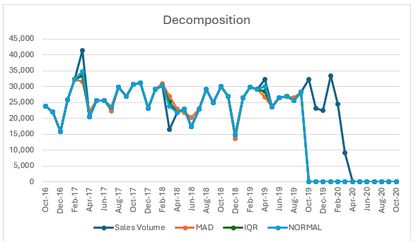
Example 3: Data preparation Method = Decomposition
Distance Estimation:
Normal:
Note: the below estimations are for comparison purposes only and are only valid when the underlying distribution is normally distributed. In your outlier analysis to the distance deviation instead of confidence limits.\ Assume data is normally distributed, the level of confidence determines the distance. For 90% confidence the distance would be 1.64 and for 95% the distance would be 1.96. This would be used as the baseline for the estimation of the distances of the methods.
Let α be there the acceptable error, then the probability of an outlier is 1-α, there is a α/2 probability that a value is higher than the acceptable upper limit. There is also α/2 probability that a value is less than the acceptable lower limit.
Let Z be the standard normal distribution and

is the number of standard deviations such there a probability of α of a random variable Z is less than

For example, Z_0.9=1.64
Central Tendency: Mean\ Dispersion: Standard deviation\ For a 2-sided analysis we have
k=Z((1-α/2))\ Z((1-α/2))=k
For the default k = 1.5, the Z_((1-α/2))=1.5\ This means 86.6% confidence and 6.7% error.
MdAD:
Central tendency: Median\ Dispersion: Median Absolute Deviation (MdAD)
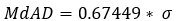
Median Absolute Deviation.

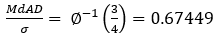
covers 50% of a standard normal distribution\ 1/2=P(|X-μ|\< MdAD)=P(|(X-μ)/σ|\<MdAD/σ)=P(|Z|\<MdAD/σ)\ P(-MdAD/σ\<Z\<MdAD/σ)=Φ(MdAD/σ)-Φ(-MdAD/σ)=2Φ(MdAD/σ)-1=1/2
Φ(MdAD/σ)=3/4

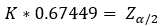
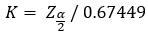
For 90% confidence we k=1.64/0.67449=2.43
For 95% confidence we k=1.96/0.67449=2.90
For the default k = 1.5, the Z_((1-α/2))=1.011735\ This means 84% confidence and 16% error.
IQR:


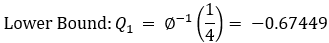
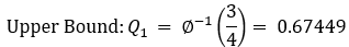
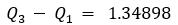
Z((1-α/2))= 0.67449+k*1.34898\ Or\ Z(α/2)= -0.67449-k*1.34898
k=(〖(Z〗_((1-α/2))-0.67449))/1.34898
For 90% confidence we have: error is 0.10\ 1.64=0.67449+k*1.34898
k=(〖(Z〗_0.95-0.67449))/1.34898
k=(1.64-0.67449)/1.34989=0.72
For 95% confidence we have: error is 0.05\ 1.96=0.67449+k*1.34898
k=(〖(Z〗_0.975-0.67449))/1.34898
k=(1.96-0.67449)/1.34989=0.95
For the default k = 1.5, the Z_((1-α/2))=2.69796\ This means 99.3% confidence and 0.3% error.
SIGMA (Mean Absolute Deviation or MAD) Method:
Central tendency: Mean\ Dispersion: Mean/Average Absolute Deviation (MAD)
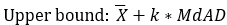
Lower bound: X ̅-k_MAD\ Upper bound: X ̅+k_MAD\ If X is normally distributed, then the ration of the absolute deviation from the Standard deviation is:
E|X-μ|/√(E(X-μ)^2 )=√(2/Π)=0.78
Z_((1-α/2))=k*0.78
k=Z_((1-α/2))/ 0.78
MAD/0.78=σ\ For 90% confidence:\ k=1.64/0.78=2.10\ For 95% confidence:
k=1.96/0.78=2.51
For the default k = 1.5, the Z_((1-α/2))=1.17\ This means 76% confidence and 12% error.
Detecting Outliers
Learn how to identify and exclude outliers in your historical data for a better forecast measurement.
{`
`}
Removing Outliers
Discover ways to remove outliers from your forecasting data sets.
{`
`}
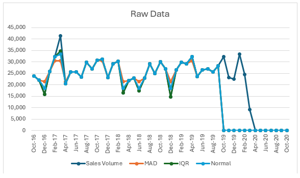
In the example below, we can see a few big spikes in the graph. These spikes are outliers. And we are more concerned with the outliers on the right side of the graph rather than the left, because these newer outliers will have an influence on our forecast.

To remove these outliers, we can go to the Forecast Method Editor and use the Outlier Detection method which uses an advanced Outlier formula.

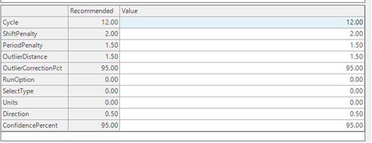
The two important parameters to know are Cycle and Outlier Distance. Cycle is your data in buckets. If your data is in monthly buckets, you will want to set this number to 12, weekly buckets is 52, etc. Outlier Distance corresponds to the standard deviation. 1.5 is the default value, however you could change to 1 standard deviation to be more aggressive in identifying outliers, or change it to 2 or 3 to be less aggressive.
Going back to the chart, we will select Outlier Detection from the Select a forecast method dropdown, and generate the forecast. Generating the forecast will perform an outlier analysis for the historic data. Clicking the Outlier Detection block in the Errors section, we can see in the chart the engine has smoothed out the history by removing all unnecessary peaks. Not only will the big spikes skew the forecast, but the little spikes could affect the forecast as well; which are sometimes not easily recognized by planners.

These results can then be published to a workbench. The workbench can then be configured to further show the outlier information easily. One such way is to set up conditional formatting where you can define rules, such as setting a condition to highlight values when your sales history is greater than 1.2 times the outlier history.

This workbench has been setup Sales History (from ERP), Outlier History (generated and published from forecast), and Adjusted History (where the historical data has been fixed and cascaded to). This along with the conditional formatting allows a planner to come in and quickly see the differences between the raw sales history and the corrected sales history.

Outlier Removal Example
When forecasting, the time series can have outliers in the data. Sometimes it is advisable to remove these overrides before doing the statistical forecast. Arkieva has a method designed to remove outliers. See screenshot below.

The system finds the outlier using the following steps. The idea is to correct the fitted value (step 2) towards the original value (original time series) up to the specified range (95% of 2 standard deviations).
Steps:
- Find out the number of data points in the time series. Call it n. We will assume n=36 in this example.
- Calculate forecast based on Robust Seasonal method using the provided time series as history
- Calculate Errors = Actuals – Forecast calculated in step 1
- Sort Errors in Ascending Order
- Find the n/4th (=9th entry in our example) error value (First Quartile)
- Find the 3n/4th (=27th entry in our example) error value (Third Quartile)
- Calculate the interquartile distance by subtracting Step 5 result from Step 6 result.
- Multiply Step 7 result by 1.5 (or the value specified in OutlierDistance Parameter of the method definition). 1.5 in this context represents two standard deviations. Call this the outlier range.
- Calculate Lower Error Bound = Step 5 result – Step 8 result
- Calculate Upper Error Bound = Step 6 result + Step 8 result
- Find any actual values from the time series that are below Step 9 result. Mark these as lower bound outliers
- Find any actual values from the time series that are above Step 10 results. Mark these as upper bound outliers
- Correct lower bound outliers by decreasing the result from step 2 by Correction Percent * Outlier Range
- Correct upper bound outliers by increasing the result from step 2 by Correction Percent * Outlier Range


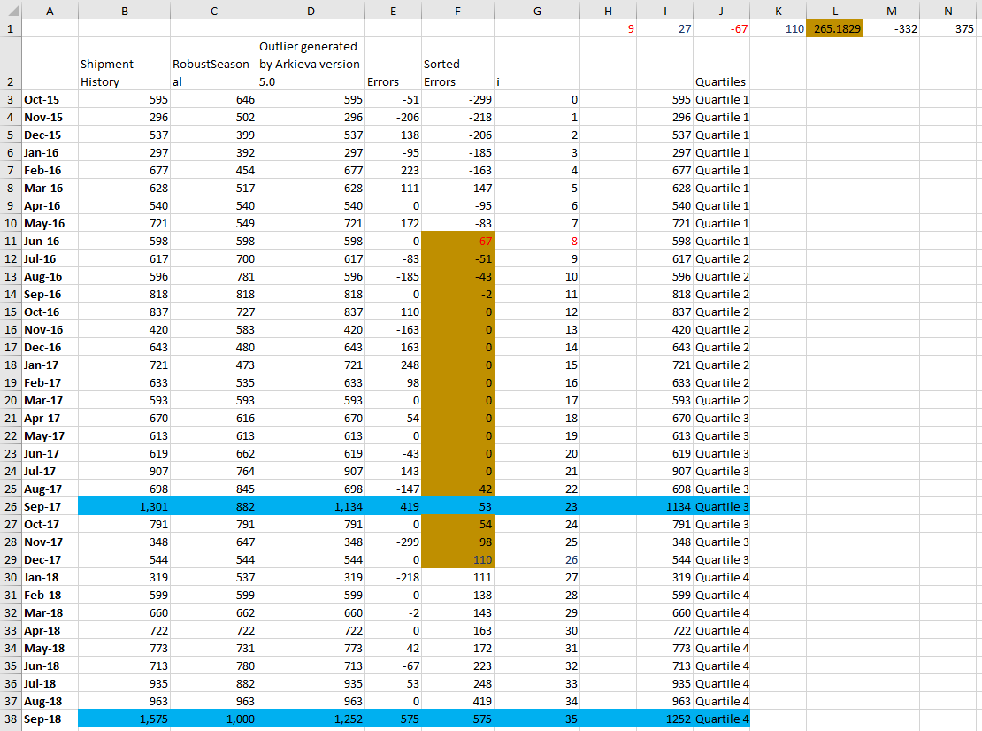
Detailed Calculations Steps
- Calculate Robust Seasonal forecast for the time series Column B; results go in column C
- Calculate errors = shipment - RobustSeasonal : Column E
- Sort Errors in Ascending Order : Column F
- Find first quartile in column F in row next to the value (G38+1)/4 in column G; G38+1 (=35+1=36 in this example) is the number of observations
- Result in cell J1
- Find third quartile in column F in row next to the value 3*(G38+1)/4 in column G
- Result in cell K1
- Calculate InterQuartile distance K1-J1 - multiply by Outlier distance parameter - store in L1; this value is 1.5 in the test; 1.5 means 2 standard deviations
- Calculate lower error bound J1 - L1 : store in M1
- Calculate upper error bound K1 + L1 : store in N1
- Produce a corrected value for any errors outside [M1,N1]
- Value is forecast Ci + CorrectionPct_(sign Error)_OutlierRange L1; Correction Pct default to 0.95 (parameter in the method)
Column 'I' was calculated in Excel based on Column 'C' from Arkieva, Column 'D' was the output from the Arkieva Outlier method. The Blue rows are the only ones that were "corrected".
Related Articles
Forecasting Terms
Time Series Any set of data which is described in terms of time. Examples: Corona Virus cases every day/week/month, etc. Sales of a smart phone over months/quarter, etc. Time Series forecasting Identifying patterns in the past and projecting them out ...Arkieva Customer Training Program
The Arkieva Customer Training Program is a customer-centric program aimed at empowering Arkieva customers with the knowledge and skills needed to harness the power of their Arkieva solution to solving complex business problems. ? Go to the bottom of ...Forecast Performance
The following is a list of Performance Metrics. Bias Total bias shows how many units your forecast is deviating from the actual sales values in absolute terms and whether the forecast is biased towards overestimating or underestimating the actual. ...Forecast Method Parameters
Each Forecast Method has unique parameters. The following are the definitions for each parameter included in the system: Alpha Affects the estimate of the intercept. Arima ArimaD: Number of times to difference the series. ArimaP: Autoregressive ...Data Anomaly Detection
Why Detect anomalies? Anomaly detection refers to the problem of finding patterns in data that do not conform to expected behavior. In the domain of supply chain management (SCM), anomaly detection is a key factor in making better forecast decisions. ...